REVIEW 3 major objections 4 minor 65 references
Optimized Sampling for Non-Line-of-Sight Imaging Using Modified Fast Fourier Transforms
T0 review · 3 major / 4 minor · reviewed 2026-08-10 · deepseek-v4-flash
Pith's one-line read Existing NLOS imaging setups oversample the relay surface, letting reconstruction work with roughly 100x fewer samples on irregular grids while keeping FFT-level speed.
desk verdict Solid NUFFT/SFFT-based NLOS algorithms with real data, but the oversampling theorem has a factor-of-two error and the 100x compression claim is not justified. read the letter →
The pith
A machine-rendered reading of the paper's core claim, the machinery that carries it, and where it could break.
The reading
What carries the argument
The load-bearing objects are the phasor field, a virtual coherent wavefront that represents the time-of-flight measurement at the relay surface; the Fresnel/paraxial approximation of a spherical phase $e^{ikr}$, which gives the slow transverse phase variation that makes lateral oversampling possible; and the sampling-ratio identity $\lambda_{sx}/\lambda_{sz} = 2|z_r - z_0|/|x_r - x_0|$ that quantifies the allowed downsampling $D$. Two modified Fourier transforms carry the algorithms: the non-uniform fast Fourier transform, which spreads irregular samples onto a dense grid, applies an FFT, and deconvolves the spreading kernel in $O(N\log N)$ work, and the scaled (fractional) FFT, which evaluates the Fourier transform on a scaled output grid using a chirp convolution with three extra FFTs. These are fused with the Rayleigh-Sommerfeld diffraction kernel to produce NURSD-1/2/3, 3D NURSD, and SRSD.
What would settle it
Reconstruct a hidden point or structured object placed close to the relay wall with large lateral offset, so $2|z_r - z_0|/|x_r - x_0| < 1$, using the downsampled-and-interpolated pipeline at short exposure time. The paper's criterion predicts visible aliasing or speckle-driven degradation in exactly that geometry; a clean reconstruction would contradict the claimed oversampling condition.
Extended reading notes
Core claim
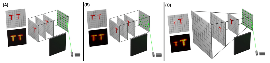
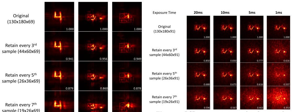
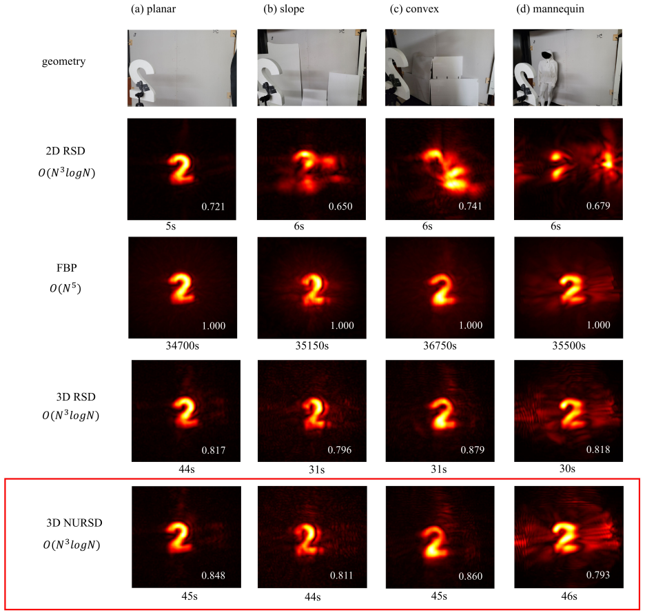
Using the phasor field formalism, the paper derives a spatial oversampling criterion for NLOS measurements. For a single point source at $(x_0,z_0)$ radiating a spherical phase wavefront, the Fresnel approximation turns the phase at relay-wall position $(x_r,z_r)$ into a quadratic term; the local transverse spatial frequency is $k(x_r-x_0)/(z_r-z_0)$, so the lateral sampling interval can be as large as $\lambda^*(z_r-z_0)/(x_r-x_0)$. Comparing that with the depth sampling interval $\lambda^*/2$ gives $\lambda_{sx}/\lambda_{sz} = 2|z_r-z_0|/|x_r-x_0| > D$, meaning the lateral axis can be downsampled by $D$ whenever the hidden object is far enough from the relay wall relative to its lateral offset. Experimental reconstructions with one out of five spatial samples retained, interpolated by nearest neighbors, give SSIM scores close to 1 against the full-data reconstruction, and the NUFFT versions reconstruct from randomly subsampled and non-uniform SPAD-array grids with quality comparable to filtered backprojection. The SRSD variant uses a scaled FFT to grow the lateral voxel size linearly with depth, matching the known resolution loss and producing perspective-correct views.
Load-bearing premise
The oversampling bound is derived for a single point source under the Fresnel/paraxial approximation with no photon noise; real scenes contain extended objects, steep angles, and shot noise, so the conclusion that the $D>1$ regime holds depends on those idealizations carrying over.
Editorial extensions
If this is right
- Relay-wall calibration no longer has to produce a uniform Cartesian grid; sparse, non-uniform, or non-planar sampling can feed the same FFT-complexity reconstruction.
- Spatial compression by a factor of about 100 (with the paper's $D=5$ and temporal bandpass) cuts the memory and readout burden of large SPAD arrays.
- Reconstruction voxels can be placed arbitrarily and coarsened with depth, so large hidden volumes can be stored and computed with about $O(Z)$ output samples instead of $O(Z^3)$ for a fixed field of view.
- The same modified-FFT trick applies to other FFT-based NLOS reconstruction algorithms, not just RSD.
- Perspective-correct reconstructions match the view from the relay wall, easing comparison with normal cameras.
Reading between the lines
- Because confocal acquisition effectively doubles the baseline sampling rate, the paper's argument implies confocal datasets lose more from aggressive downsampling than non-confocal ones, which the authors note matches prior observations.
- The oversampling bound also suggests an adaptive-sampling rule: spend pixels on near-field, small-offset regions where $D$ is smaller, and sparsely sample regions far from the relay wall.
- Replacing the naive interpolation step with photon-noise-aware denoising or learned reconstruction should extend the compression benefit to low-exposure acquisitions, where the paper's own results show the simple scheme fails.
- If the Fresnel/paraxial assumption is relaxed, the same sampling-ratio derivation should produce a generalized $D$ that depends on angle, giving a testable prediction for non-paraxial relay geometries.
Editorial analysis
A structured set of objections, weighed in public.
Referee Report
Summary. The paper proposes three families of modifications to the standard Rayleigh-Sommerfeld Diffraction (RSD) algorithm for non-line-of-sight (NLOS) imaging: Scaled RSD (SRSD), which changes the lateral voxel size with depth using a scaled Fourier transform; Non-Uniform RSD (NURSD-1/2/3), which uses the NUFFT to allow non-uniform sampling of the relay surface and of the reconstruction grid; and 3D NURSD for non-planar relay surfaces. The central theoretical claim is that existing NLOS relay-surface measurements are spatially oversampled, formalized as lambda_{sx}/lambda_{sz} = 2|z_r-z_0|/|x_r-x_0| > D (Eq. 25/57). This is used to justify spatial subsampling and interpolation, leading to a claimed ~100x data reduction. The algorithms are validated on public datasets and on a custom 16x16 SPAD-array acquisition, with comparisons to standard RSD and filtered backprojection.
Significance. If the oversampling claim holds, the paper provides both a theoretical explanation for the empirically observed compressibility of NLOS measurements and practical tools to exploit it, while preserving FFT-level computational complexity. The SRSD additionally provides a memory-efficient, perspective-correct reconstruction volume. The manuscript gives detailed derivations of the SFFT and NUFFT variants, uses public datasets and external baselines, and demonstrates the algorithms on real non-planar relay surfaces and a real SPAD array. These strengths make the work potentially useful to the NLOS imaging community. The main caveat is that the central sampling-rate derivation is too optimistic by a factor of two and lacks a worst-case analysis for extended scenes, so the quantitative scope of the compression claim needs revision.
major comments (3)
- [Supplement A.3, Eqs. (54)-(57)] The derivation equates the local phase slope k'' = k(x_r-x_0)/(2(z_r-z_0)) with the transverse spatial frequency, but the instantaneous frequency of the quadratic Fresnel phase phi(x_r) = k(x_r-x_0)^2/(2(z_r-z_0)) is dphi/dx_r = k(x_r-x_0)/(z_r-z_0) = 2k''. For a finite relay aperture, the relevant Nyquist bound is set by the maximum of this frequency over the aperture, not by its value at a single local coordinate. The corrected bound is lambda_{sx} <= lambda*(z_r-z_0)/(2 max|x_r-x_0|), which makes the oversampling ratio in Eq. (25) and Eq. (57) too large by a factor of about two. With the paper's own geometry (1.8 m x 1.3 m wall, lambda_c = 4 cm, depths 1-3 m), the admissible D values in Table 1 shrink accordingly, and the '~100x' data-reduction claim in Sections 1.1 and 7.2.3 is not supported for scene points at moderate lateral offsets. The empirical reconstructions remain useful evidence, but the mathematical justification for 'typically oversample' is not established as stated.
- [Section 5 and Supplement A.3] The sampling criterion is derived for a single paraxial point source. Real hidden scenes contain extended objects at multiple depths and lateral positions, so the required sampling rate is determined by the worst-case combination of maximum lateral offset and minimum depth over all points contributing to the measurement. The paper does not provide such a worst-case analysis, and the statement in Section 1.1 that 'most NLOS imaging setups currently oversample' is therefore not quantitatively justified for general scenes. The authors should either supply a worst-case derivation or explicitly restrict the claim to scenes satisfying specified geometric bounds.
- [Section 7.2.1 and Fig. 9] The paper correctly states that the sampling derivation ignores photon noise and demonstrates experimentally that interpolation degrades sharply at low exposure times. However, the abstract and Section 1.1 present spatial oversampling and 'roughly 100x less data' as general properties without this caveat. The compression claim should be explicitly conditioned on sufficient photon flux and on the geometric conditions from the corrected sampling criterion, so that readers do not take the unqualified statement as the paper's central result.
minor comments (4)
- [Section 5, step 3] The interpolation protocol says 'Reconstruct using fast RSD algorithm, with the wavelength set to 2 lambda_s', but the experiments in Section 7.2 use lambda_c = 4 cm with 1 cm sampling; the relationship between lambda_s and lambda_c in this step should be clarified.
- [Section 8.1, Fig. 13] The text refers to a 'low pass filter' applied to compute the blue SSIM scores, but does not specify the filter parameters or implementation; please provide details.
- [Eq. (2)] The integrals over domega and dvec{x}_p are written without explicit limits; adding the integration ranges would improve reproducibility.
- [General notation] The symbol N is used both for the side length of the reconstruction cube and for the number of samples per dimension; defining these separately would avoid confusion in Sections 3.1, 4.2, and 6.
Circularity Check
No significant circularity: the oversampling criterion is a parameter-free physical derivation, and the NUFFT/SFFT algorithms are validated against external baselines and public datasets.
full rationale
The paper's load-bearing claim—that NLOS relay surfaces are typically oversampled—is derived in Supplement A.3 from a stated point-source model and Fresnel/paraxial approximation (Eqs. 45-57), not fitted to the paper's own reconstructions. The ratio λsx/λsz = 2|zr−z0|/|xr−x0| (Eq. 57) is a mathematical consequence of the assumed phase model; it does not presuppose the conclusion. The NUFFT and SFFT algorithms are standard external tools, and NURSD/SRSD are compared against independent RSD and FBP reconstructions on public datasets. Citations to the authors' prior phasor-field work [12-14] supply the physical model and are not invoked as a uniqueness theorem to forbid alternatives. The paper itself flags the Poisson-noise limitation (Sec. 7.2.1), which affects applicability but not circularity. A potential factor-of-two concern in the instantaneous-frequency step of Eq. 55 is a correctness/mathematical issue, not a case of the result being equivalent to its inputs by construction. Overall, the derivation chain is self-contained.
Assumptions & free parameters
free parameters (3)
- alpha (and beta) lateral scaling factors =
not reported; values between 0 and 1
- lambda_c phasor field center wavelength =
for example 4 cm; varied over a range in experiments
- D downsampling ratio =
D = 2, 4, 5 in the examples
assumptions (6)
- domain assumption The NLOS transient measurement is modeled with the phasor-field framework and reconstructed by the Rayleigh-Sommerfeld diffraction integral (Eq. 2).
- domain assumption The hidden scene can be represented as a sum of bandlimited point sources, P(k)=0 for k >= |k*|, each radiating e^{ikr} (Supplement A.3).
- domain assumption The paraxial/Fresnel approximation is valid, r approx (z-z0)+(x-x0)^2/[2(z-z0)] (Supplement Eq. 52).
- ad hoc to paper Photon (Poisson) noise can be ignored for the sampling-rate derivation.
- ad hoc to paper NUFFT approximation error is negligible because the imaging system oversamples the relay surface.
- standard math Helmholtz reciprocity and separability of RSD allow swapping illumination and detection and plane-to-plane propagation.
Cite this review
Pith. "Pith review of Optimized Sampling for Non-Line-of-Sight Imaging Using Modified Fast Fourier Transforms." pith.science (2026). https://pith.science/paper/4SEIDU3F
@misc{pith2026250105244,
  author       = {Pith},
  title        = {Pith review of: Optimized Sampling for Non-Line-of-Sight Imaging Using Modified Fast Fourier Transforms},
  year         = {2026},
  howpublished = {\url{https://pith.science/paper/4SEIDU3F}},
  note         = {Machine review of arXiv:2501.05244}
}
read the original abstract
Non-line-of-Sight (NLOS) imaging systems collect light at a diffuse relay surface and input this measurement into computational algorithms that output a 3D volumetric reconstruction. These algorithms utilize the Fast Fourier Transform (FFT) to accelerate the reconstruction process but require both input and output to be sampled spatially with uniform grids. However, the geometry of NLOS imaging inherently results in non-uniform sampling on the relay surface when using multi-pixel detector arrays, even though such arrays significantly reduce acquisition times. Furthermore, using these arrays increases the data rate required for sensor readout, posing challenges for real-world deployment. In this work, we utilize the phasor field framework to demonstrate that existing NLOS imaging setups typically oversample the relay surface spatially, explaining why the measurement can be compressed without significantly sacrificing reconstruction quality. This enables us to utilize the Non-Uniform Fast Fourier Transform (NUFFT) to reconstruct from sparse measurements acquired from irregularly sampled relay surfaces of arbitrary shapes. Furthermore, we utilize the NUFFT to reconstruct at arbitrary locations in the hidden volume, ensuring flexible sampling schemes for both the input and output. Finally, we utilize the Scaled Fast Fourier Transform (SFFT) to reconstruct larger volumes without increasing the number of samples stored in memory. All algorithms introduced in this paper preserve the computational complexity of FFT-based methods, ensuring scalability for practical NLOS imaging applications.
Figures


Figures from the paper (17 more)






Reference graph
Works this paper leans on
-
[1]
D. Faccio, A. Velten, and G. Wetzstein, “Non-line-of-sight imaging,” Nature Reviews Physics , vol. 2, no. 6, pp. 318–327, Jun. 2020, number: 6 Publisher: Nature Publishing Group. [Online]. Available: https://www.nature.com/articles/s42254-020-0174-8 1
work page 2020
-
[2]
Non-line-of-sight imaging using phasor-field virtual wave optics,
X. Liu, I. Guilln, M. La Manna, J. H. Nam, S. A. Reza, T. Huu Le, A. Jarabo, D. Gutierrez, and A. Velten, “Non-line-of-sight imaging using phasor-field virtual wave optics,” Nature, vol. 572, no. 7771, pp. 620–623, Aug. 2019, number: 7771 Publisher: Nature Publishing Group. [Online]. Available: https://www.nature.com/articles/s41586-019-1461-3 1, 3, 6, 14
work page 2019
-
[3]
Phasor field diffraction based reconstruction for fast non-line-of-sight imaging systems,
X. Liu, S. Bauer, and A. Velten, “Phasor field diffraction based reconstruction for fast non-line-of-sight imaging systems,” Nature Communications, vol. 11, no. 1, pp. 1–13, Apr. 2020, number: 1 Publisher: Nature Publishing Group. [Online]. Available: https://www.nature.com/articles/s41467-020-15157-4 1, 2, 3, 5, 6, 9, 14, 19
work page 2020
-
[4]
Low-latency time-of-flight non-line-of-sight imaging at 5 frames per second,
J. H. Nam, E. Brandt, S. Bauer, X. Liu, M. Renna, A. Tosi, E. Sifakis, and A. Velten, “Low-latency time-of-flight non-line-of-sight imaging at 5 frames per second,” Nature Communications , vol. 12, no. 1, p. 6526, Dec. 2021. [Online]. Available: https://www.nature.com/articles/s41467-021-26721-x 1, 3, 5, 14, 19
work page 2021
-
[5]
Fast-Gated 16 1 SPAD Array for Non-Line-of-Sight Imaging Applications,
M. Renna, J. H. Nam, M. Buttafava, F. Villa, A. Velten, and A. Tosi, “Fast-Gated 16 1 SPAD Array for Non-Line-of-Sight Imaging Applications,” Instruments, vol. 4, no. 2, p. 14, Jun. 2020, number: 2 Publisher: Multidisciplinary Digital Publishing Institute. [Online]. Available: https://www.mdpi.com/2410-390X/4/2/14 1
work page 2020
-
[6]
S. Riccardo, E, Conca, V. Sesta, A. Velten, and A. Tosi, “Fast-Gated 16 16 SPAD Array with 16 on-chip 6 ps Time-to-Digital Converters for Non-Line-of-Sight Imaging,” IEEE Sensors Journal , pp. 1–1, 2022. 1, 4
work page 2022
-
[7]
Dynamic non-line-of-sight imaging system based on the optimization of point spread functions,
C. Pei, A. Zhang, Y. Deng, F. Xu, J. Wu, D. U.-L. Li, H. Qiao, L. Fang, and Q. Dai, “Dynamic non-line-of-sight imaging system based on the optimization of point spread functions,” Optics Express , vol. 29, no. 20, pp. 32 349–32 364, Sep. 2021, publisher: Optica Publishing Group. [Online]. Available: https://opg.optica.org/oe/abstract.cfm?uri=oe-29-20-32349 1, 3
work page 2021
-
[8]
Confocal non-line-of-sight imaging based on the light-cone transform,
M. OToole, D. B. Lindell, and G. Wetzstein, “Confocal non-line-of-sight imaging based on the light-cone transform,” Nature, vol. 555, no. 7696, pp. 338–341, Mar. 2018. [Online]. Available: https://www.nature.com/articles/nature25489 1, 2, 3
work page 2018
Show all 65 references
-
[9]
Wave-based non-line-of-sight imaging using fast f-k migration,
D. B. Lindell, G. Wetzstein, and M. O’Toole, “Wave-based non-line-of-sight imaging using fast f-k migration,” ACM Transactions on Graphics , vol. 38, no. 4, pp. 1–13, Aug. 2019. [Online]. Available: https://dl.acm.org/doi/10.1145/3306346.3322937 1, 3
2019
-
[10]
Paraxial theory of phasor-field imaging,
J. Dove and J. H. Shapiro, “Paraxial theory of phasor-field imaging,” Optics Express, vol. 27, no. 13, pp. 18 016– 18 037, Jun. 2019. [Online]. Available: https://www.osapublishing.org/oe/abstract.cfm?uri=oe-27-13-18016 2, 3, 6
2019
-
[11]
The Fractional Fourier Transform and Applications,
D. H. Bailey and P. N. Swarztrauber, “The Fractional Fourier Transform and Applications,” SIAM Review , vol. 33, no. 3, pp. 389–404, Sep. 1991, publisher: Society for Industrial and Applied Mathematics. [Online]. Available: https://epubs.siam.org/doi/10.1137/1033097 2, 7
1991 doi
-
[12]
Phasor field waves: experimental demonstrations of wave-like properties,
S. A. Reza, M. La Manna, S. Bauer, and A. Velten, “Phasor field waves: experimental demonstrations of wave-like properties,” Optics Express , vol. 27, no. 22, p. 32587, Oct. 2019. [Online]. Available: https://www.osapublishing.org/abstract.cfm?URI=oe-27-22-32587 2, 3, 6 21
2019
-
[13]
Phasor field waves: A Huygens-like light transport model for non-line-of-sight imaging applications,
S. A. Reza, M. L. Manna, S. Bauer, A. Velten, and A. Velten, “Phasor field waves: A Huygens-like light transport model for non-line-of-sight imaging applications,” Optics Express , vol. 27, no. 20, pp. 29 380–29 400, Sep. 2019, publisher: Optical Society of America. [Online]. ...
2019
-
[14]
Phasor field waves: a mathematical treatment,
J. A. Teichman, “Phasor field waves: a mathematical treatment,” Optics Express , vol. 27, no. 20, pp. 27 500–27 506, Sep. 2019, publisher: Optical Society of America. [Online]. Available: https: //www.osapublishing.org/oe/abstract.cfm?uri=oe-27-20-27500 2, 3
2019
-
[15]
Recovering three-dimensional shape around a corner using ultrafast time-of-flight imaging,
A. Velten, T. Willwacher, O. Gupta, A. Veeraraghavan, M. G. Bawendi, and R. Raskar, “Recovering three-dimensional shape around a corner using ultrafast time-of-flight imaging,” Nature Communications , vol. 3, p. 745, Mar. 2012. [Online]. Available: https://www.nature.com/artic...
2012
-
[16]
Fast back-projection for non-line of sight reconstruction,
V. Arellano, D. Gutierrez, and A. Jarabo, “Fast back-projection for non-line of sight reconstruction,” Optics Express, vol. 25, no. 10, pp. 11 574–11 583, May 2017. [Online]. Available: https://www.osapublishing.org/oe/ abstract.cfm?uri=oe-25-10-11574 3
2017
-
[17]
Convolutional Approximations to the General Non-Line-of-Sight Imaging Operator,
B. Ahn, A. Dave, A. Veeraraghavan, I. Gkioulekas, and A. Sankaranarayanan, “Convolutional Approximations to the General Non-Line-of-Sight Imaging Operator,” in 2019 IEEE/CVF International Conference on Computer Vision (ICCV) . Seoul, Korea (South): IEEE, Oct. 2019, pp. 7888–78...
2019
-
[18]
Diffuse Mirrors: 3D Reconstruction from Diffuse Indirect Illumination Using Inexpensive Time-of-Flight Sensors,
F. Heide, L. Xiao, W. Heidrich, and M. B. Hullin, “Diffuse Mirrors: 3D Reconstruction from Diffuse Indirect Illumination Using Inexpensive Time-of-Flight Sensors,” in 2014 IEEE Conference on Computer Vision and Pattern Recognition . Columbus, OH, USA: IEEE, Jun. 2014, pp. 3222...
2014
-
[19]
Error Backprojection Algorithms for Non-Line-of-Sight Imaging,
M. L. Manna, F. Kine, E. Breitbach, J. Jackson, T. Sultan, and A. Velten, “Error Backprojection Algorithms for Non-Line-of-Sight Imaging,” IEEE Transactions on Pattern Analysis and Machine Intelligence , pp. 1–1, 2018. 3
2018
-
[20]
Beyond Volumetric Albedo A Surface Optimization Framework for Non-Line-Of-Sight Imaging,
C.-Y. Tsai, A. C. Sankaranarayanan, and I. Gkioulekas, “Beyond Volumetric Albedo A Surface Optimization Framework for Non-Line-Of-Sight Imaging,” in 2019 IEEE/CVF Conference on Computer Vision and Pattern Recognition (CVPR) . Long Beach, CA, USA: IEEE, Jun. 2019, pp. 1545–1555...
2019
-
[21]
SNLOS: Non-line-of-sight Scanning through Temporal Focusing,
A. Pediredla, A. Dave, and A. Veeraraghavan, “SNLOS: Non-line-of-sight Scanning through Temporal Focusing,” in 2019 IEEE International Conference on Computational Photography (ICCP), May 2019, pp. 1–13, iSSN: 2472-
2019
-
[22]
Non-line-of-sight Imaging with Partial Occluders and Surface Normals,
F. Heide, M. OToole, K. Zang, D. B. Lindell, S. Diamond, and G. Wetzstein, “Non-line-of-sight Imaging with Partial Occluders and Surface Normals,” ACM Transactions on Graphics , vol. 38, no. 3, pp. 1–10, Jun. 2019. [Online]. Available: https://dl.acm.org/doi/10.1145/3269977 3
2019 doi
-
[23]
Non-line-of-sight Reconstruction Using Efficient Transient Rendering,
J. Iseringhausen and M. B. Hullin, “Non-line-of-sight Reconstruction Using Efficient Transient Rendering,” ACM Transactions on Graphics , vol. 39, no. 1, pp. 8:1–8:14, Jan. 2020. [Online]. Available: https://doi.org/10.1145/3368314 3
2020 doi
-
[24]
Non-line-of-sight reconstruction with signalobject collaborative regularization,
X. Liu, J. Wang, Z. Li, Z. Shi, X. Fu, and L. Qiu, “Non-line-of-sight reconstruction with signalobject collaborative regularization,” Light: Science & Applications , vol. 10, no. 1, p. 198, Dec. 2021. [Online]. Available: https://www.nature.com/articles/s41377-021-00633-3 3, 5, 14
2021
-
[25]
Non-line-of-sight imaging with arbitrary illumination and detection pattern,
X. Liu, J. Wang, L. Xiao, Z. Shi, X. Fu, and L. Qiu, “Non-line-of-sight imaging with arbitrary illumination and detection pattern,” Nature Communications , vol. 14, no. 1, p. 3230, Jun. 2023. [Online]. Available: https://www.nature.com/articles/s41467-023-38898-4 3, 4, 19
2023
-
[26]
Non-Line-of-Sight Surface Reconstruction Using the Directional Light-Cone Transform,
S. I. Young, D. B. Lindell, B. Girod, D. Taubman, and G. Wetzstein, “Non-Line-of-Sight Surface Reconstruction Using the Directional Light-Cone Transform,” in 2020 IEEE/CVF Conference on Computer Vision and Pattern Recognition (CVPR) . Seattle, W A, USA: IEEE, Jun. 2020, pp. 14...
2020
-
[27]
Efficient Non-Line-of-Sight Imaging from Transient Sinograms,
M. Isogawa, D. Chan, Y. Yuan, K. Kitani, and M. OToole, “Efficient Non-Line-of-Sight Imaging from Transient Sinograms,” in Computer Vision ECCV 2020 , A. Vedaldi, H. Bischof, T. Brox, and J.-M. Frahm, Eds. Cham: Springer International Publishing, 2020, vol. 12352, pp. 193–208,...
2020 doi
-
[28]
Optical Non-Line-of-Sight Physics-Based 3D Human Pose Estimation,
M. Isogawa, Y. Yuan, M. O’Toole, and K. Kitani, “Optical Non-Line-of-Sight Physics-Based 3D Human Pose Estimation,” in 2020 IEEE/CVF Conference on Computer Vision and Pattern Recognition (CVPR) . Seattle, W A, USA: IEEE, Jun. 2020, pp. 7011–7020. [Online]. Available: https://i...
2020
-
[29]
Paraxial phasor-field physical optics,
J. Dove and J. H. Shapiro, “Paraxial phasor-field physical optics,” Optics Express , vol. 28, no. 14, pp. 21 095–21 109, Jul. 2020, publisher: Optical Society of America. [Online]. Available: https://www.osapublishing.org/oe/abstract.cfm?uri=oe-28-14-21095 3, 6
2020
-
[30]
Nonparaxial phasor-field propagation,
——, “Nonparaxial phasor-field propagation,” Optics Express , vol. 28, no. 20, pp. 29 212–29 229, Sep. 2020, publisher: Optical Society of America. [Online]. Available: https://www.osapublishing.org/oe/abstract.cfm? uri=oe-28-20-29212 3
2020
-
[31]
Speckled speckled speckle,
——, “Speckled speckled speckle,” Optics Express, vol. 28, no. 15, pp. 22 105–22 120, Jul. 2020, publisher: Optical Society of America. [Online]. Available: https://www.osapublishing.org/oe/abstract.cfm?uri=oe-28-15-22105 3
2020
-
[32]
Towards a more accurate light transport model for non-line-of-sight imaging,
T. Sultan, S. A. Reza, and A. Velten, “Towards a more accurate light transport model for non-line-of-sight imaging,” Optics Express , vol. 32, no. 5, pp. 7731–7761, Feb. 2024, publisher: Optica Publishing Group. [Online]. Available: https://opg.optica.org/oe/abstract.cfm?uri=o...
2024
-
[33]
The role of Wigner Distribution Function in Non-Line-of-Sight Imaging,
X. Liu and A. Velten, “The role of Wigner Distribution Function in Non-Line-of-Sight Imaging,” in 2020 IEEE International Conference on Computational Photography (ICCP) , Apr. 2020, pp. 1–12, iSSN: 2472-7636. 3
2020
-
[34]
Virtual Mirrors: Non-Line-of-Sight Imaging Beyond the Third Bounce,
D. Royo, T. Sultan, A. Muoz, K. Masumnia-Bisheh, E. Brandt, D. Gutierrez, A. Velten, and J. Marco, “Virtual Mirrors: Non-Line-of-Sight Imaging Beyond the Third Bounce,” ACM Transactions on Graphics, vol. 42, no. 4, pp. 140:1–140:15, Jul. 2023. [Online]. Available: https://dl.a...
2023 doi
-
[35]
Analysis of Feature Visibility in Non-Line-Of-Sight Measurements,
X. Liu, S. Bauer, and A. Velten, “Analysis of Feature Visibility in Non-Line-Of-Sight Measurements,” in 2019 IEEE/CVF Conference on Computer Vision and Pattern Recognition (CVPR) . Long Beach, CA, USA: IEEE, Jun. 2019, pp. 10 132–10 140. [Online]. Available: https://ieeexplore...
2019
-
[36]
Virtual Light Transport Matrices for Non-Line-of-Sight Imaging,
J. Marco, A. Jarabo, J. H. Nam, X. Liu, M. . Cosculluela, A. Velten, and D. Gutierrez, “Virtual Light Transport Matrices for Non-Line-of-Sight Imaging,” in 2021 IEEE/CVF International Conference on Computer Vision (ICCV), Oct. 2021, pp. 2420–2429, iSSN: 2380-7504. 3
2021
-
[37]
Non-line-of-sight-imaging using dynamic relay surfaces,
M. L. Manna, J.-H. Nam, S. A. Reza, A. Velten, and A. Velten, “Non-line-of-sight-imaging using dynamic relay surfaces,” Optics Express, vol. 28, no. 4, pp. 5331–5339, Feb. 2020, publisher: Optica Publishing Group. [Online]. Available: https://opg.optica.org/oe/abstract.cfm?uri...
2020
-
[38]
Fast Non-line-of-sight Imaging with Non- planar Relay Surfaces,
C. Gu, T. Sultan, K. Masumnia-Bisheh, L. Waller, and A. Velten, “Fast Non-line-of-sight Imaging with Non- planar Relay Surfaces,” in 2023 IEEE International Conference on Computational Photography (ICCP) , Jul. 2023, pp. 1–12, iSSN: 2472-7636. 3, 6, 19
2023
-
[39]
Non-Line-of-Sight Imaging With Signal Superresolution Network,
J. Wang, X. Liu, L. Xiao, Z. Shi, L. Qiu, and X. Fu, “Non-Line-of-Sight Imaging With Signal Superresolution Network,” 2023, pp. 17 420–17 429. [Online]. Available: https://openaccess.thecvf.com/content/CVPR2023/ html/Wang Non-Line-of-Sight Imaging With Signal Superresolution N...
2023
-
[40]
Deep Non-line-of-sight Imaging from Under-scanning Measurements,
Y. Li, Y. Zhang, J. Ye, F. Xu, and Z. Xiong, “Deep Non-line-of-sight Imaging from Under-scanning Measurements,” Nov. 2023. [Online]. Available: https://openreview.net/forum?id=JCN9YsZiwB 4
2023
-
[41]
Learning to Enhance Aperture Phasor Field for Non-Line-of-Sight Imaging,
I. Cho, H. Shim, and S. J. Kim, “Learning to Enhance Aperture Phasor Field for Non-Line-of-Sight Imaging,” Jul. 2024, arXiv:2407.18574 [cs]. [Online]. Available: http://arxiv.org/abs/2407.18574 4, 14, 19
2024 arXiv
-
[42]
Compressed sensing for active non-line-of-sight imaging,
J.-T. Ye, X. Huang, Z.-P. Li, and F. Xu, “Compressed sensing for active non-line-of-sight imaging,” Optics Express, vol. 29, no. 2, p. 1749, Jan. 2021. [Online]. Available: https://opg.optica.org/abstract.cfm?URI= oe-29-2-1749 4
2021
-
[43]
Digital holography and its multidimensional imaging applications: a review,
T. Tahara, X. Quan, R. Otani, Y. Takaki, and O. Matoba, “Digital holography and its multidimensional imaging applications: a review,” Microscopy, vol. 67, no. 2, pp. 55–67, 02 2018. [Online]. Available: https://doi.org/10.1093/jmicro/dfy007 4
2018 doi
-
[44]
Computer-generated holograms for 3d imaging: A survey,
E. Sahin, E. Stoykova, J. M¨ akinen, and A. Gotchev, “Computer-generated holograms for 3d imaging: A survey,” ACM Comput. Surv. , vol. 53, no. 2, Mar. 2020. [Online]. Available: https://doi.org/10.1145/3378444 4
2020 doi
-
[45]
Shifted Fresnel diffraction for computational holography,
R. P. Muffoletto, J. M. Tyler, and J. E. Tohline, “Shifted Fresnel diffraction for computational holography,” Optics Express , vol. 15, no. 9, pp. 5631–5640, Apr. 2007, publisher: Optica Publishing Group. [Online]. Available: https://opg.optica.org/oe/abstract.cfm?uri=oe-15-9-5631 4
2007
-
[46]
Nonuniform sampled scalar diffraction calculation using nonuniform fast Fourier transform,
T. Shimobaba, T. Kakue, M. Oikawa, N. Okada, Y. Endo, R. Hirayama, and T. Ito, “Nonuniform sampled scalar diffraction calculation using nonuniform fast Fourier transform,” Optics Letters , vol. 38, no. 23, pp. 5130–5133, Dec. 2013, publisher: Optica Publishing Group. [Online]....
2013
-
[47]
J. W. Goodman, Introduction to Fourier optics , 3rd ed. Englewood, Colo: Roberts & Co, 2005, oCLC: ocm56632414. 4 23
2005
-
[48]
Robust Monte Carlo Methods For Light Transport Simulation,
E. Veach, “Robust Monte Carlo Methods For Light Transport Simulation,” PhD thesis, Stanford University , Dec. 1997. 5
1997
-
[49]
Dual Photography,
P. Sen, B. Chen, G. Garg, S. R. Marschner, M. Horowitz, M. Levoy, and H. P. A. Lensch, “Dual Photography,” in ACM SIGGRAPH 2005 Papers , ser. SIGGRAPH ’05. New York, NY, USA: ACM, 2005, pp. 745–755. [Online]. Available: http://doi.acm.org/10.1145/1186822.1073257 5
2005
-
[50]
M. Born, E. Wolf, and A. B. Bhatia, Principles of optics: electromagnetic theory of propagation, interference, and diffraction of light, seventh (expanded) anniversary edition, 60th anniversary edition ed. Cambridge: Cambridge University Press, 2019. 6
2019
-
[51]
A linear filtering approach to the computation of discrete fourier transform,
L. Bluestein, “A linear filtering approach to the computation of discrete fourier transform,” IEEE Transactions on Audio and Electroacoustics, vol. 18, no. 4, pp. 451–455, 1970. 7
1970
-
[52]
Bagchi and S
S. Bagchi and S. K. Mitra, The Nonuniform Discrete Fourier Transform and Its Applications in Signal Processing. Boston, MA: Springer US, 1999. [Online]. Available: http://link.springer.com/10.1007/978-1-4615-4925-3 11
1999 doi
-
[53]
Fast Fourier Transforms for Nonequispaced Data,
A. Dutt and V. Rokhlin, “Fast Fourier Transforms for Nonequispaced Data,” SIAM Journal on Scientific Computing, vol. 14, no. 6, pp. 1368–1393, Nov. 1993, publisher: Society for Industrial and Applied Mathematics. [Online]. Available: https://epubs.siam.org/doi/abs/10.1137/0914...
1993 doi
-
[54]
Fast Fourier Transforms for Nonequispaced Data, II,
——, “Fast Fourier Transforms for Nonequispaced Data, II,” Applied and Computational Harmonic Analysis , vol. 2, no. 1, pp. 85–100, Jan. 1995. [Online]. Available: https://www.sciencedirect.com/science/article/pii/ S106352038571007X 11, 12
1995
-
[55]
Accelerating the Nonuniform Fast Fourier Transform,
L. Greengard and J.-Y. Lee, “Accelerating the Nonuniform Fast Fourier Transform,” SIAM Review , vol. 46, no. 3, pp. 443–454, Jan. 2004. [Online]. Available: http://epubs.siam.org/doi/10.1137/S003614450343200X 11, 12
2004 doi
-
[56]
A note on fast Fourier transforms for nonequispaced grids,
G. Steidl, “A note on fast Fourier transforms for nonequispaced grids,” Advances in Computational Mathematics, vol. 9, no. 3, pp. 337–352, Nov. 1998. [Online]. Available: https://doi.org/10.1023/A:1018901926283 11, 12
1998 doi
-
[57]
A Parallel Nonuniform Fast Fourier Transform Library Based on an Exponential of Semicircle
A. H. Barnett, J. Magland, and L. af Klinteberg, “A Parallel Nonuniform Fast Fourier Transform Library Based on an Exponential of Semicircle” Kernel,” SIAM Journal on Scientific Computing , vol. 41, no. 5, pp. C479–C504, Jan. 2019, publisher: Society for Industrial and Applied...
2019 doi
-
[58]
Aliasing error of the exp( β √ 1 − z2) kernel in the nonuniform fast fourier transform,
A. H. Barnett, “Aliasing error of the exp( β √ 1 − z2) kernel in the nonuniform fast fourier transform,” Applied and Computational Harmonic Analysis , vol. 51, pp. 1–16, 2021. [Online]. Available: https: //www.sciencedirect.com/science/article/pii/S1063520320300725 11, 12
2021
-
[59]
cuFINUFFT: a load-balanced GPU library for general-purpose nonuniform FFTs,
Y.-h. Shih, G. Wright, J. Andn, J. Blaschke, and A. H. Barnett, “cuFINUFFT: a load-balanced GPU library for general-purpose nonuniform FFTs,” in 2021 IEEE International Parallel and Distributed Processing Symposium Workshops (IPDPSW) , Jun. 2021, pp. 688–697. [Online]. Availab...
2021
-
[60]
Uniform error estimates for nonequispaced fast Fourier transforms,
D. Potts and M. Tasche, “Uniform error estimates for nonequispaced fast Fourier transforms,” Sampling Theory, Signal Processing, and Data Analysis , vol. 19, no. 2, p. 17, Nov. 2021. [Online]. Available: https://doi.org/10.1007/s43670-021-00017-z 11, 12
2021 doi
-
[61]
Nonuniform fast Fourier transforms using min-max interpolation,
J. Fessler and B. Sutton, “Nonuniform fast Fourier transforms using min-max interpolation,” IEEE Transactions on Signal Processing , vol. 51, no. 2, pp. 560–574, Feb. 2003, conference Name: IEEE Transactions on Signal Processing. [Online]. Available: https://ieeexplore.ieee.or...
2003
-
[62]
Onsite Non-Line-of-Sight Imaging via Online Calibration,
Z. Pan, R. Li, T. Gao, Z. Wang, S. Shen, P. Liu, T. Wu, J. Yu, and S. Li, “Onsite Non-Line-of-Sight Imaging via Online Calibration,” IEEE Photonics Journal , vol. 14, no. 5, pp. 1–11, Oct. 2022, conference Name: IEEE Photonics Journal. 14
2022
-
[63]
Compressive Single-Photon 3D Cameras,
F. Gutierrez-Barragan, A. Ingle, T. Seets, M. Gupta, and A. Velten, “Compressive Single-Photon 3D Cameras,” 2022, pp. 17 854–17 864. [Online]. Available: https://openaccess.thecvf.com/content/CVPR2022/ html/Gutierrez-Barragan Compressive Single-Photon 3D Cameras CVPR 2022 pape...
2022
-
[64]
Efficient high-order accurate Fresnel diffraction via areal quadrature and the nonuniform fast Fourier transform,
A. H. Barnett, “Efficient high-order accurate Fresnel diffraction via areal quadrature and the nonuniform fast Fourier transform,” Journal of Astronomical Telescopes, Instruments, and Systems , vol. 7, no. 02, Jan. 2021. [Online]. Available: https://www.spiedigitallibrary. org...
2021 doi
-
[65]
Iterating the transient light transport matrix for non-line-of-sight imaging,
T. Sultan, E. Brandt, K. Masumnia-Bisheh, S. Riccardo, P. Polynkin, A. Tosi, and A. Velten, “Iterating the transient light transport matrix for non-line-of-sight imaging,” 2024. [Online]. Available: https://arxiv.org/abs/2412.10300 6 24 Optimized Sampling for Non-Line-of-Sight...
2024 arXiv
Reviewed August 10, 2026 · model on record in the stance chip above.
Discussion (0). Continue with ORCID to comment.