Problem hardness of diluted Ising models: Population Annealing versus Simulated Annealing

Diego Porras; Fernando Mart\'inez-Garc\'ia

REVIEW 3 major objections 5 minor 1 cited by

Problem hardness of diluted Ising models: Population Annealing versus Simulated Annealing

T0 review · 3 major / 5 minor · reviewed 2026-08-10 · deepseek-v4-flash

Challenge this review Re-run · record.json Download PDF Read on arXiv ↗ Review JSON

Pith's one-line read Finding ground states of diluted Sherrington–Kirkpatrick Ising models is hardest when spins have about 1.8 interactions on average, and population annealing is the more efficient heuristic in that regime.

desk verdict A careful empirical benchmark showing PA beats SA near a hardness peak in diluted SK, but the hardness metrics are PA-internal and the finite-size scaling is thinner than it looks. read the letter →

arxiv 2501.07638 v2 pith:ZQXXQZUY submitted 2025-01-13 cond-mat.stat-mech cond-mat.dis-nn

Fernando Martínez-García , Diego Porras This is my paper · ORCID

classification cond-mat.stat-mechcond-mat.dis-nn

keywords populationannealingsimulateddilutedSherrington-KirkpatrickmodelErdős–Rényigraphsspinglassgroundstateseasy-hard-easytransitionproblemhardnessadaptivetemperatureschedule

verification ladder T0 review T1 audit T2 compute T3 formal

The pith

A machine-rendered reading of the paper's core claim, the machinery that carries it, and where it could break.

The reading

The paper studies the diluted Sherrington–Kirkpatrick Ising model, a spin glass whose spin couplings sit on random Erdős–Rényi graphs of tunable average degree $Np$, from sparse graphs up to the fully connected SK limit. It claims to find an easy-hard-easy transition in how hard it is to locate ground states: hardness rises as the graph becomes more dilute, peaks at an extrapolated $Np \approx 1.8$, and then falls again. The peak is explained by the competition between clusterization and connectivity in the underlying graph: small isolated clusters are easy, a merging giant component is hardest, and higher connectivity inside that component makes the problem easy again. Near the peak, population annealing finds ground states with substantially less computational work than an optimally tuned simulated annealing, while both perform similarly in the easy limits. The paper further claims that an adaptive inverse-temperature schedule for population annealing is more robust against miscalibrated final temperatures and slightly more efficient near the peak than a linear schedule.

What carries the argument

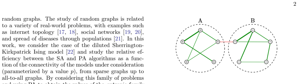
The argument is carried by two diagnostics extracted from a single population-annealing run: the mean square family size $\rho_t = \lim_{R\to\infty} R \sum_i n_i^2$ and the effective population size $R_{\text{eff}} = \sigma^2(E)/\sigma^2_{\bar{E}}(E)$, computed from jackknife variance estimates. Both measure how aggressively the resampling step prunes the population; large $\rho_t$ and small $R_{\text{eff}}$ indicate a rugged free-energy landscape and hence a hard instance. These quantities locate the hardness peak as a function of $Np$ and are compared against the giant-component size of the Erdős–Rényi graph. The mechanistic claim is then tested on clusterized regular graphs, in which clusters of size $S$ and degree $D$ are varied independently, isolating clusterization (size) from connectivity (degree) as the two competing controls of hardness.

What would settle it

Compute an exact time-to-solution for simulated annealing with optimized hyperparameters on the same class of diluted SK instances at larger sizes (e.g., $N=400$ or beyond), using an exact solver to certify ground states, and test whether the TTS peak occurs at $Np \approx 1.7$–$1.8$ as the $N\to\infty$ extrapolation predicts; if the TTS peak is absent, displaced, or disappears when the PA diagnostics are replaced by direct success-probability measurements, the claimed transition is an artifact of the $\rho_t$/$R_{\text{eff}}$ proxies.

Watch

Extended reading notes

Core claim

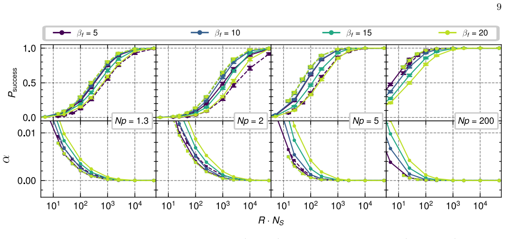
The central discovery is that problem hardness in the diluted Sherrington–Kirkpatrick Ising model, measured through the population-annealing diagnostics $\rho_t$ (mean square family size) and $R_{\text{eff}}$ (effective population size), is not monotone in the graph connectivity $p$. Instead, hardness follows an easy-hard-easy curve as a function of $Np$, with a maximum at $Np \simeq 1.7$–$1.8$ in the infinite-size limit, extrapolated from sizes $N=300,400,500$. The authors attribute this transition to the structure of the underlying Erdős–Rényi graphs: at low $Np$ the graph breaks into small independent clusters that are individually easy to solve; as $Np$ grows past the percolation threshold these clusters merge into a giant component, producing weakly coupled clusters that trap single-spin-flip algorithms in local minima; at larger $Np$, the higher internal connectivity removes those traps and hardness drops. This mechanism is tested directly on clusterized regular graphs, where hardness increases with cluster size and peaks at degree $D=3$ before declining. In efficiency benchmarks on $N=200$ instances, population annealing outperforms an optimally calibrated simulated annealing near the hardness peak (e.g., at $Np=2$) for both success probability and approximation ratio, while achieving similar efficiency at the $p=1$ SK limit and at the dilute $Np=1.3$ side.

Load-bearing premise

The load-bearing premise is that the population-annealing diagnostics $\rho_t$ and $R_{\text{eff}}$ faithfully measure the algorithmic difficulty of finding ground states for this model family; if they do not correlate with true time-to-solution, the easy-hard-easy transition and its peak position could be artifacts of the resampling dynamics rather than intrinsic problem hardness.

Editorial extensions

If this is right

Near the hardness peak at $Np\approx 2$, population annealing requires less computational work than simulated annealing to reach ground states, so PA is the better heuristic for intermediate-connectivity spin-glass problems.
The extrapolated peak at $Np \approx 1.7$–$1.8$ gives benchmark designers a target regime where random spin-glass instances are hardest, useful for stress-testing new optimization algorithms.
The log-inverse Gaussian fit to the $\rho_t$ distribution means that near the peak the instance-to-instance difficulty spread widens, so budgets adequate for the average instance will fail on a non-negligible fraction of hard instances.
The adaptive temperature schedule removes the need to calibrate the final inverse temperature as long as it is high enough, making population annealing effectively hyperparameter-free in this respect.
PA's advantage over SA disappears at both easy limits ($p=1$ and very dilute $Np$), consistent with the resampling step mattering only when the free-energy landscape is rugged though not fully connected.

Reading between the lines

Editorial extensions of the paper, not claims the author makes directly.

If the $\rho_t$–TTS correlation holds beyond the sizes tested, a single short PA run could serve as a cheap hardness predictor, letting a practitioner allocate more compute to the hard tail of instances flagged by high $\rho_t$.
The location of the hardness peak just above the Erdős–Rényi percolation threshold ($Np=1$) suggests that other NP-hard problems on sparse random graphs (e.g., Max-Cut or random $k$-SAT) may exhibit a similar easy-hard-easy pattern tuned by a percolation-like connectivity parameter; that is a testable extension.
The finite-size scaling $Np_{\max}(N) = (Np)_{\max,\infty} + A/N^\nu$ with $\nu \approx 0.8$ raises the question, not settled in the paper, of whether the hardness peak is a genuine critical phenomenon or a finite-size crossover; resolving this would require larger sizes and a scaling collapse.

Share X Bluesky LinkedIn Reddit HN

Editorial analysis

A structured set of objections, weighed in public.

Desk editor's note, referee report, and a circularity audit.

Desk Editor's Note

read the letter

You should know this paper is a solid empirical benchmark, not a breakthrough. The easy-hard-easy transition in diluted SK was already in Perera et al. (Ref. [35]), and the authors say so. What they add is a PA-focused characterization via family-size metrics, a mechanistic story built from clusterized regular graphs, and a fair PA-vs-SA efficiency comparison with optimized SA hyperparameters. That last part is the strongest contribution: they use Gurobi for three of the four Np values, report both success probability and approximation ratio, and show PA clearly wins at Np=2, which is near their hardness peak.

The simulation design is careful: 6000 instances for each hardness data point, bootstrap errors on the peak fits, and explicit attention to thermalization via R>100ρt. The mechanism study with clusterized regular graphs in Fig. 6 is a nice controlled probe of the cluster-size and connectivity effects. The adaptive schedule robustness result is useful for practitioners.

Soft spots, in proportion. The central hardness measure is ρ_t and R_eff, both computed from a single PA run. The paper argues these correlate with TTS via prior work, but there is no independent calibration for diluted SK. That matters because the transition peak is located with these metrics. The direct TTS check at N=200 uses only four Np values (1.3, 2, 5, 200), so it brackets the peak but does not localize it. This is a real limitation, though the paper does not overclaim precision there. The finite-size extrapolation of the peak via Eq. (12) fits three parameters to three sizes; that is not a test of the scaling law. The quoted asymptotic value Np≈1.77 is a rough estimate, and the authors essentially say so. Also, the Np=200 ground states come from PA rather than an exact solver; they checked no lower energy appeared, which is reasonable but not a proof. Finally, no code or data are released, only "available upon request."

None of this sinks the paper. The existence of a hardness peak near Np≈2 is visible in the raw data, and the direct efficiency comparison gives independent support that something hard is happening there. The paper is honest, well-parameterized, and does not oversell its mechanistic explanation. It deserves a serious referee.

My recommendation: send it to peer review. Ask the authors to release code and data, and to either calibrate ρ_t against TTS for a few sizes or soften the claim that it faithfully tracks problem hardness. The three-point fit should be presented as an extrapolation, not a verification.

Referee Report

3 major / 5 minor

Summary. The paper studies the diluted Sherrington-Kirkpatrick Ising model using population annealing (PA) and characterizes problem hardness through two PA-derived quantities, the mean square family size ρ_t and the effective population size R_eff. From these, the authors report an easy-hard-easy transition in hardness as the average degree Np varies, with the hardness peak extrapolating to Np≈1.77 (ρ_t) and Np≈1.68 (R_eff), and they associate this behavior with the clusterization and connectivity of the underlying Erdős-Rényi graphs. The paper then compares PA with simulated annealing (SA) on N=200 instances at Np=1.3, 2, 5, and 200, finding that PA outperforms SA near the claimed hardness peak. Finally, an adaptive inverse-temperature schedule for PA is shown to be more efficient and more robust to final-temperature miscalibration than a linear schedule.

Significance. If the central claim holds, the paper identifies a nonmonotonic hardness landscape in a physically and combinatorially relevant family of Ising models and provides practical guidance on when population annealing is preferable to simulated annealing. The computational study is carefully set up: it uses 6000 instances for the hardness data, optimizes SA hyperparameters to avoid straw-man comparisons, and uses multiple metrics (ρ_t, R_eff, success probability, approximation ratio). The adaptive-schedule comparison is a useful practical contribution. However, the central hardness transition is defined through PA-internal metrics rather than an external measure of optimization difficulty, and the direct efficiency benchmark is too sparse to confirm the precise location of the peak. These issues are fixable but currently leave the main claim only partially supported.

major comments (3)

[Section III, Figs. 2-4] The easy-hard-easy transition is characterized exclusively by the PA-internal quantities ρ_t and R_eff, both computed from the family-size statistics of a single PA run, so their co-peaking is not an independent confirmation of a problem-hardness transition. The correlations with time-to-solution and autocorrelation cited in Refs. [23,24,35] were established for other model families, and no calibration is provided for the diluted SK model studied here. The central claim would be substantially strengthened by validating ρ_t (or R_eff) against an independent hardness measure, such as the SA time-to-solution or integrated autocorrelation time, on the same instances over a fine range of Np.
[Section III, Eq. (12) and Fig. 4] The finite-size extrapolation of the peak position uses exactly three system sizes (N=300, 400, 500) for a three-parameter fit (asymptotic value, amplitude, and exponent), so the quoted power-law form is not tested and the bootstrap errors do not include the uncertainty in the functional form. The asymptotic peak values 1.77±0.03 and 1.68±0.01 should be presented as rough estimates, and the statement that the dependence could indicate critical behavior is premature without additional sizes.
[Section IV A, Figs. 8-9] The direct efficiency comparison samples only four values of Np (1.3, 2, 5, 200), which is too coarse to locate the time-to-solution maximum or to verify that the efficiency peak coincides with the ρ_t peak near Np≈1.7-1.8. In addition, for Np=200 the reference ground states are obtained from PA itself rather than from an exact solver, which introduces a possible circularity in the benchmark. Additional Np values around the claimed peak and an independent verification of the reference energies are needed to support the conclusion that PA outperforms SA specifically near the hardness peak.

minor comments (5)

[Section III, Fig. 6] The clusterized regular-graph model shows a hardness peak at degree D=3, but no quantitative link is established between D and the mean degree Np of the Erdős-Rényi graphs; the diluted SK peak occurs near Np≈1.7-1.8, not at D=3. A mapping or a discussion of why D=3 corresponds to the ER peak would make the clusterization/connectivity association more convincing.
[Section II C, Eq. (7)] The culling fraction is introduced as ε in the text but appears as ϵ in Eq. (7); the notation should be unified.
[Section IV A, Fig. 9] The statement that SA and PA reach similar efficiencies in the SK limit depends on the PA sweep count: PA with NS=1 is similar to SA, but PA with NS=5 or 10 is noticeably worse, so the conclusion should be qualified as depending on PA hyperparameters.
[Section III, Table I and Fig. 7] The quality of the log-inverse Gaussian fits is not quantified; the claim of perfect agreement would be supported by reporting goodness-of-fit statistics or confidence bands.
[Overall] The manuscript states that data are available upon request but does not provide a repository; for a computational study, releasing instance generation code and data would improve reproducibility.

Circularity Check

0 steps flagged · score 1.0 of 10

No significant circularity: the easy-hard-easy transition is an observed behavior of externally grounded PA diagnostics, and the SA-vs-PA comparison is checked against Gurobi exact ground states.

full rationale

The central easy-hard-easy claim is an observed behavior of the PA-derived diagnostics rho_t and R_eff, not a quantity fitted to itself. These diagnostics are defined in prior work (Refs. [23,24,35]) and are cited as correlating with time-to-solution and autocorrelation; the paper does not redefine TTS in terms of them. The efficiency comparison in Section IV A is an independent check: for Np = 1.3, 2, and 5, exact ground states are obtained with the Gurobi optimizer, and SA hyperparameters are optimized before comparing with PA. The observed TTS and approximation-ratio behavior at N = 200 qualitatively supports the hardness peak near Np = 2. The clusterized regular graph study in Section III is a mechanism test using the same rho_t diagnostic, but it varies independent graph properties (cluster size S and degree D) and is not an input to the diluted-SK measurement. Self-citations (Refs. [5,14,38]) concern contextual applications, hyperparameter discussion, and implementation of systematic resampling; none carries the central claim. The three-parameter fit of Eq. (12) to three system sizes (N = 300, 400, 500) yields an extrapolated peak but with zero degrees of freedom; this is a statistical limitation, and the paper itself notes that 'A more accurate estimation of those values could be obtained by performing more simulations and increasing the size of the problem instances,' but this is not a circular reduction. No equation is equivalent to its own input by construction. Score 1 reflects only the presence of minor, non-load-bearing self-citations.

Assumptions & free parameters 9 free parameters · 6 assumptions · 0 invented entities

The central results are empirical. They depend on fitted scaling parameters, a chosen culling fraction, and the validity of PA-based hardness metrics. No new physical or algorithmic entities are introduced.

free parameters (9)

Asymptotic hardness peak (N p)_max for ρ_t = 1.77 ± 0.03
Extrapolated from finite-size scaling fit of peak positions of log(ρ_t); Eq. (12) and Fig. 4.
Scaling amplitude A_t = 25.9 ± 4.4
Fitted in Eq. (12) for ρ_t peak positions.
Scaling exponent ν_t = 0.83 ± 0.05
Fitted in Eq. (12) for ρ_t peak positions.
Asymptotic hardness peak (N p)_max for R_eff = 1.68 ± 0.01
Extrapolated from finite-size scaling fit of peak positions of log(R_eff).
Scaling amplitude A_R = 4.7 ± 1.6
Fitted in Eq. (12) for R_eff peak positions.
Scaling exponent ν_R = 0.79 ± 0.1
Fitted in Eq. (12) for R_eff peak positions.
Log-inverse Gaussian distribution parameters (l, μ, λ) = See Table I
Fitted to histograms of log10(ρ_t) for each N and p; used to describe hardness distribution.
Culling fraction ε = 0.085
Chosen for adaptive schedule in Section IV B; controls resampling fraction per temperature step.
Minimum replicas R_min = 15
Set for adaptive schedule to estimate energy standard deviation reliably.

assumptions (6)

standard math Metropolis-Hastings single-spin-flip updates converge to the Boltzmann distribution at each fixed temperature
Invoked in Section II B to justify annealing sweeps.
standard math Systematic resampling provides unbiased estimates of the target distribution in population annealing
Used in Section II C to justify the resampling step.
domain assumption Mean square family size ρ_t and effective population size R_eff are valid measures of thermalization and problem hardness
Relied on throughout Section III to define the easy-hard-easy transition; supported by prior correlations in Refs. [23,24,35].
domain assumption The percolation properties of Erdős-Rényi graphs (giant component at N p>1) determine the clusterization that drives hardness
Used in Section III to explain the hardness peak; tested indirectly with clusterized regular graphs.
domain assumption Gurobi Optimizer returns exact ground states for N=200 instances with N p=1.3, 2, 5
Used in Section IV A as reference energies for TTS computation.
domain assumption PA with R=10^5, NT=100, NS=20 finds true ground states for N p=200 instances
Used in Section IV A to obtain target energies when Gurobi is too slow; checked by absence of lower-energy configurations.

how reviews work

0 comments

Cite this review

Pith. "Pith review of Problem hardness of diluted Ising models: Population Annealing versus Simulated Annealing." pith.science (2026). https://pith.science/paper/ZQXXQZUY

@misc{pith2026250107638,
  author       = {Pith},
  title        = {Pith review of: Problem hardness of diluted Ising models: Population Annealing versus Simulated Annealing},
  year         = {2026},
  howpublished = {\url{https://pith.science/paper/ZQXXQZUY}},
  note         = {Machine review of arXiv:2501.07638}
}

read the original abstract

Population annealing is a variant of the simulated annealing algorithm that improves the quality of the thermalization process in systems with rough free-energy landscapes by introducing a resampling process. We consider the diluted Sherrington-Kirkpatrick Ising model using population annealing to study its efficiency in finding solutions to combinatorial optimization problems. From this study, we find an easy-hard-easy transition in the model hardness as the problem instances become more diluted, and associate this behaviour to the clusterization and connectivity of the underlying Erd\H{o}s-R\'enyi graphs. We calculate the efficiency of obtaining minimum energy configurations and find that population annealing outperforms simulated annealing for the cases close to this hardness peak while reaching similar efficiencies in the easy limits. Finally, it is known that population annealing can be used to define an adaptive inverse temperature annealing schedule. We compare this adaptive method to a linear schedule and find that the adaptive method achieves improved efficiencies while being robust against final temperature miscalibrations.

Figures

Figures reproduced from arXiv: 2501.07638 by the authors.

**Figure 4.** FIG. 4. Results of the fit from Eq. ( [PITH_FULL_IMAGE:figures/full_fig_p005_4.png] view at source ↗

**Figure 3.** FIG. 3. Mean value of the logarithm of [PITH_FULL_IMAGE:figures/full_fig_p005_3.png] view at source ↗

Figures from the paper (4 more)

**Figure 6.** Figure 6: FIG. 6. Study of the problem hardness of clusterized regular [PITH_FULL_IMAGE:figures/full_fig_p006_6.png]

**Figure 8.** Figure 8: FIG. 8. Mean value of the TTS obtained over 10 [PITH_FULL_IMAGE:figures/full_fig_p007_8.png]

**Figure 9.** Figure 9: FIG. 9. Probability of finding the ground state, [PITH_FULL_IMAGE:figures/full_fig_p008_9.png]

**Figure 10.** Figure 10: FIG. 10. Probability of finding the ground state, [PITH_FULL_IMAGE:figures/full_fig_p009_10.png]

Discussion (0). Continue with ORCID to comment.

Forward citations

Cited by 1 Pith paper

Reviewed papers in the Pith corpus that reference this work. Sorted by Pith novelty score. Full citation record

Optimised Feature Subset Selection via Simulated Annealing
cs.LG 2025-07 conditional novelty 4.0 of 10

SA-FDR uses simulated annealing guided by the Fisher discriminant ratio to find compact feature subsets for logistic regression, often beating RFE and Lasso on sparsity with comparable AUC.

Reference graph

Works this paper leans on

44 extracted references · 39 canonical work pages · cited by 1 Pith paper

[35]

Perera, F

D. Perera, F. Hamze, J. Raymond, M. Weigel, and H. G. Katzgraber, Physical Review E 101, 023316 (2020)

work page 2020
[1]

ˇCern´ y, Journal of Optimization Theory and Applica- tions 45, 41 (1985)

V. ˇCern´ y, Journal of Optimization Theory and Applica- tions 45, 41 (1985)

work page 1985
[2]

D. S. Johnson, in International colloquium on automata, languages, and programming (Springer, 1990) pp. 446– 461

work page 1990
[3]

Mansini and M

R. Mansini and M. G. Speranza, European Journal of Operational Research 114, 219 (1999)

work page 1999
[4]

Crama and M

Y. Crama and M. Schyns, European Journal of Opera- tional Research 150, 546 (2003)

work page 2003
[5]

Fern´ andez-Lorenzo, J

´Alvaro Rubio-Garc ´ ıa, S. Fern´ andez-Lorenzo, J. J. Garc ´ ıa- Ripoll, and D. Porras, Physica A: Statistical Mechanics and its Applications 639, 129637 (2024)

work page 2024
[6]

S. F. Edwards and P. W. Anderson, Journal of Physics F: Metal Physics 5, 965 (1975)

1975
[7]

M´ ezard, G

M. M´ ezard, G. Parisi, and M. A. Virasoro,Spin glass the- ory and beyond: An Introduction to the Replica Method and Its Applications , Vol. 9 (World Scientific Publishing Company, 1987)

work page 1987

Show all 44 references

[8]

Barahona, Journal of Physics A: Mathematical and General 15, 3241 (1982)

F. Barahona, Journal of Physics A: Mathematical and General 15, 3241 (1982)

1982
[9]

Jaum` a, J

G. Jaum` a, J. J. Garc ´ ıa-Ripoll, and M. Pino, Advanced Quantum Technologies 7, 2300245 (2024)

2024
[10]

Kirkpatrick, C

S. Kirkpatrick, C. D. Gelatt Jr, and M. P. Vecchi, Science 220, 671 (1983)

1983
[11]

R. H. Swendsen and J.-S. Wang, Physical Review Letters 57, 2607 (1986)

1986
[12]

Hukushima and Y

K. Hukushima and Y. Iba, in AIP Conference Proceed- ings, Vol. 690 (American Institute of Physics, 2003) pp. 200–206

2003
[13]

Machta, Physical Review E 82, 026704 (2010)

J. Machta, Physical Review E 82, 026704 (2010)

2010
[14]

´Alvaro Rubio-Garc ´ ıa, J. J. Garc ´ ıa-Ripoll, and D. Porras, arXiv preprint arXiv:2210.00807 (2022)

2022 arXiv
[15]

C. P. Robert, G. Casella, and G. Casella, Monte Carlo statistical methods, Vol. 2 (Springer, 1999)

1999
[16]

W. Wang, J. Machta, and H. G. Katzgraber, Physical Review E 92, 013303 (2015)

2015
[17]

Albert, H

R. Albert, H. Jeong, and A.-L. Barab´ asi, Nature 401, 130 (1999)

1999
[18]

Faloutsos, P

M. Faloutsos, P. Faloutsos, and C. Faloutsos, ACM SIG- COMM computer communication review 29, 251 (1999)

1999
[19]

M. E. Newman, D. J. Watts, and S. H. Strogatz, Pro- ceedings of the national academy of sciences 99, 2566 (2002)

2002
[20]

Robins, T

G. Robins, T. Snijders, P. Wang, M. Handcock, and P. Pattison, Social networks 29, 192 (2007). 11

2007
[21]

M. E. Newman, Physical Review E 66, 016128 (2002)

2002
[22]

Boettcher, Physical Review Letters 124, 177202 (2020)

S. Boettcher, Physical Review Letters 124, 177202 (2020)

2020
[23]

W. Wang, J. Machta, and H. G. Katzgraber, Physical Review E 92, 063307 (2015)

2015
[24]

Amey and J

C. Amey and J. Machta, Physical Review E 97, 033301 (2018)

2018
[25]

Erd˝ os and A

P. Erd˝ os and A. R´ enyi, Publicationes Mathematicae De- brecen 6, 18 (1959)

1959
[26]

Erd˝ os, A

P. Erd˝ os, A. R´ enyi,et al., Publ. Math. Inst. Hung. Acad. Sci 5, 17 (1960)

1960
[27]

Bollob´ as,Random Graphs (Springer, 1998)

B. Bollob´ as,Random Graphs (Springer, 1998)

1998
[28]

Frieze and M

A. Frieze and M. Karo´ nski, Introduction to random graphs (Cambridge University Press, 2015)

2015
[29]

L. Y. Barash, M. Weigel, M. Borovsk` y, W. Janke, and L. N. Shchur, Computer Physics Communications 220, 341 (2017)

2017
[30]

Sherrington and S

D. Sherrington and S. Kirkpatrick, Physical Review Let- ters 35, 1792 (1975)

1975
[31]

Svenson, Physical Review E 64, 036122 (2001)

P. Svenson, Physical Review E 64, 036122 (2001)

2001
[32]

H. G. Katzgraber, in Journal of Physics: Conference Se- ries, Vol. 95 (IOP Publishing, 2008) p. 012004

2008
[33]

Weigel, Physical Review E—Statistical, Nonlinear, and Soft Matter Physics 76, 066706 (2007)

M. Weigel, Physical Review E—Statistical, Nonlinear, and Soft Matter Physics 76, 066706 (2007)

2007
[34]

T. F. Rønnow, Z. Wang, J. Job, S. Boixo, S. V. Isakov, D. Wecker, J. M. Martinis, D. A. Lidar, and M. Troyer, science 345, 420 (2014)

2014
[36]

Doucet, N

A. Doucet, N. De Freitas, and N. Gordon, Sequential Monte Carlo methods in practice , 3 (2001)

2001
[37]

Gessert, W

D. Gessert, W. Janke, and M. Weigel, Physical Review E 108, 065309 (2023)

2023
[38]

Mart ´ ınez-Garc ´ ıa, F

F. Mart ´ ınez-Garc ´ ıa, F. R. F. Pereira, and P. Parrado- Rodr ´ ıguez, arXiv preprint arXiv:2405.03776 (2024)

2024 arXiv
[39]

Barzegar, F

A. Barzegar, F. Hamze, C. Amey, and J. Machta, Phys- ical Review E 109, 065301 (2024)

2024
[40]

Weigel, L

M. Weigel, L. Barash, L. Shchur, and W. Janke, Physical Review E 103, 053301 (2021)

2021
[41]

Efron and R

B. Efron and R. J. Tibshirani, An introduction to the bootstrap (Chapman and Hall/CRC, 1994)

1994
[42]

Yucesoy, J

B. Yucesoy, J. Machta, and H. G. Katzgraber, Physical Review E 87, 012104 (2013)

2013
[43]

Gurobi Optimizer Refer- ence Manual,

Gurobi Optimization, LLC, “Gurobi Optimizer Refer- ence Manual,” (2024)

2024
[44]

P. L. Ebert, D. Gessert, and M. Weigel, Physical Review E 106, 045303 (2022)

2022

Pith tools

Reviewed August 10, 2026 · model on record in the stance chip above.

[1] [35]

Perera, F

D. Perera, F. Hamze, J. Raymond, M. Weigel, and H. G. Katzgraber, Physical Review E 101, 023316 (2020)

work page 2020

[2] [1]

ˇCern´ y, Journal of Optimization Theory and Applica- tions 45, 41 (1985)

V. ˇCern´ y, Journal of Optimization Theory and Applica- tions 45, 41 (1985)

work page 1985

[3] [2]

D. S. Johnson, in International colloquium on automata, languages, and programming (Springer, 1990) pp. 446– 461

work page 1990

[4] [3]

Mansini and M

R. Mansini and M. G. Speranza, European Journal of Operational Research 114, 219 (1999)

work page 1999

[5] [4]

Crama and M

Y. Crama and M. Schyns, European Journal of Opera- tional Research 150, 546 (2003)

work page 2003

[6] [5]

Fern´ andez-Lorenzo, J

´Alvaro Rubio-Garc ´ ıa, S. Fern´ andez-Lorenzo, J. J. Garc ´ ıa- Ripoll, and D. Porras, Physica A: Statistical Mechanics and its Applications 639, 129637 (2024)

work page 2024

[7] [6]

S. F. Edwards and P. W. Anderson, Journal of Physics F: Metal Physics 5, 965 (1975)

1975

[8] [7]

M´ ezard, G

M. M´ ezard, G. Parisi, and M. A. Virasoro,Spin glass the- ory and beyond: An Introduction to the Replica Method and Its Applications , Vol. 9 (World Scientific Publishing Company, 1987)

work page 1987