REVIEW 4 major objections 5 minor 48 references
Adaptive-depth randomized measurement for fermionic observables
T0 review · 4 major / 5 minor · reviewed 2026-08-10 · deepseek-v4-flash
Pith's one-line read This paper introduces an adaptive-depth fermionic classical shadow protocol and claims that the required depth for approximating a fermionic observable $H$ scales as $\max\{d_{\mathrm{int}}(H)^2/\log n,\ d_{\mathrm{int}}(H)\}$ while…
desk verdict Good new idea about adaptive-depth fermionic shadows, but the sample-complexity guarantee is average-case and rests on unproven sign and factorization assumptions; the abstract overclaims. read the letter →
The pith
A machine-rendered reading of the paper's core claim, the machinery that carries it, and where it could break.
The reading
What carries the argument
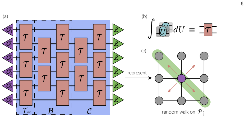
The load-bearing object is the tensor-network representation of the $d$-depth matchgate shadow channel. Each independent two-qubit matchgate is replaced by a fixed fourth-order tensor obtained from the second-moment twirl of the matchgate group, and connecting these tensors in the brickwork architecture produces a tensor network whose contraction gives $\alpha_{S,d} = \langle\langle 0,0|\mathcal{C}|\gamma_S,\gamma_S\rangle\rangle$. For two-local Majorana strings the contraction is then shown to evolve as a symmetry lazy random walk on a polynomial space; the walk's transition probabilities yield a closed-form Poisson-sum expression for the dominant part $\alpha^L_{S,d}$, and an auxiliary remainder bound relates $\alpha^L_{S,d}$ to $\alpha_{S,d}$. The adaptive depth rule follows from requiring $\alpha^L_{S,d}=\Omega(1/\mathrm{poly}(n))$.
What would settle it
Prepare a fixed computational-basis state or an adversarially chosen state and run ADFCS at depth $d^*$, measuring the empirical variance of $\mathrm{Tr}(\hat\rho\gamma_S)$; if the variance exceeds $1/\alpha_{S,d}$ by more than a constant factor, the sample-complexity claim as stated fails. A second check is to compute the remainder coefficients $R_{i,j}(\mu,\nu,t)$ for an adjacent Majorana pair at shallow depth: a positive diagonal remainder or a negative off-diagonal remainder violates the assumption behind the proof of the depth rule.
Extended reading notes
Core claim
The paper's central claim is that the depth needed for a random matchgate measurement is set by the observable's interaction distance, not by the system size. For a $k$-local Majorana string $\gamma_S$ with constant $k$ and interaction distance $d_{\mathrm{int}}(S)=O(\log n)$, a random circuit of depth $d=\Theta(\log n)$ already makes the shadow eigenvalue $\alpha_{S,d}$ polynomially large, i.e. $\alpha_{S,d}=\Omega(1/\mathrm{poly}(n))$; more generally the required depth is $d^*=\Theta(\max\{d_{\mathrm{int}}(S)^2/\log n,\ d_{\mathrm{int}}(S)\})$. Because the variance of the estimation is bounded by $1/\alpha_{S,d}$, this gives the same order of sample complexity as the original FCS protocol while using far shallower circuits.
Load-bearing premise
The depth guarantee and the matching sample complexity rest on the variance bound $\mathrm{Var}[v]\le 1/\alpha_{S,d}$, which is derived by averaging the unknown state over the uniform (Haar) distribution; a fixed adversarial state could require more samples than the stated order.
Editorial extensions
If this is right
- A fermionic Hamiltonian whose terms have logarithmic interaction distance can be measured with $O(\log n)$-depth random matchgate circuits and polynomial sample complexity.
- Shallow-depth estimation preserves the unbiasedness of the classical-shadow estimator whenever $\alpha_{S,d}\neq 0$.
- For a 10-qubit Kitaev chain, depth $d=3$ already suffices to reach estimation errors comparable with the full FCS protocol.
- For observables with interaction distance $d_{\mathrm{int}}=\omega(\log n)$, the required depth interpolates between logarithmic and polynomial scaling as the observable becomes more nonlocal.
- The sample-complexity bound retains the form $O(1/(\alpha_{S,d}\epsilon^2))$, matching the original FCS order when $\alpha_{S,d}$ is polynomially large.
Reading between the lines
- The same tensor-network-to-random-walk reduction could be re-derived for other circuit geometries, such as non-brickwork or open-boundary matchgate layouts, changing only the kernel of the walk and hence the constants in the depth rule.
- A state-dependent version of the variance bound would be needed before using ADFCS for adversarial or worst-case inputs; the current protocol's practical guarantee is tied to the Haar-averaged variance.
- The per-term depth selection suggests a practical variational-quantum-eigensolver-style measurement strategy: choose a different measurement depth for each Hamiltonian term according to its own $d_{\mathrm{int}}$, rather than one global depth.
- The closed-form Poisson-sum formula could be turned into a lookup table or analytic depth selector, removing the numerical-fitting step and giving a fully deterministic protocol.
Formalized claims in Lean
-
Claim #1: The paper's central claim is that the depth needed for a random matchgate measurement is set by the observable's interaction distance, not by the system size. For a $k$-local Majorana string $\gamma_S$ with constant $k$ and interaction distance $d_{\mathrm{int}}(S)=O(\log n)$, a random circuit of depth $d=\Theta(\log n)$ already makes the shadow eigenvalue $\alpha_{S,d}$ polynomially large, i.e. $
/-- @claim 1 The paper's central claim is that the depth needed for a random matchgate measurement is set by the observable's interaction distance, not by the system size. For a $k$-local Majorana string $\gamma_S$ with constant $k$ and interaction distance $d_{\mathrm{int}}(S)=O(\log n)$, a random circuit of depth $d=\Theta(\log n)$ already makes the shadow eigenvalue $\alpha_{S,d}$ polynomially large, i.e. $ -/
def central_claim : Prop :=
Editorial analysis
A structured set of objections, weighed in public.
Referee Report
Summary. The paper introduces an adaptive-depth fermionic classical shadow (ADFCS) protocol. The protocol uses d-depth brickwork random matchgate circuits and adapts the depth to the observable H via its interaction distance d_int(H). The central claim is that, for k-local Majorana observables with d_int(H)=O(log n), depth d* = Θ(max{d_int(H)^2/log n, d_int(H)}) suffices to keep the key parameter α_{S,d} at order Ω(1/poly(n)), while maintaining the same order of sample complexity as the full matchgate FCS protocol. The analysis maps the tensor-network contraction for α_{S,d} to a random walk on a polynomial space, derives an analytical Poisson-summation formula for the 2-local case, and proposes a factorization ansatz for the k-local case. Numerical experiments on random states and on the Kitaev chain Hamiltonian support the depth-vs-accuracy tradeoff.
Significance. If the main claim holds, the paper addresses a concrete open question: whether a shallow-depth FCS protocol can match the sample complexity of the full-depth FCS protocol for a meaningful class of fermionic observables. The tensor-network-to-random-walk mapping and the closed-form Poisson approximation for α_{S,d} are valuable technical contributions, and the Kitaev-chain demonstration is a nice practical illustration. However, the central result is conditional: the 2-local lower bound rests on an unproven sign assumption, the k-local extension rests on a numerically validated ansatz rather than a proof, and the sample-complexity statement is derived for Haar-averaged states. These gaps limit the strength of the conclusions that can be drawn from the paper in its current form.
major comments (4)
- [Appendix G, Theorem 1 and Eq. (G30)] The 2-local lower bound α_{S,d} ≥ (47/72) max_{d'≤d} α^L_{S,d'} is derived under the sign-definiteness assumption R_{ij}(μ,μ,t) ≤ 0 and R_{ij}(μ,ν,t) ≥ 0 for μ≠ν, which is only supported by the numerical sign plot in Fig. 8. If this assumption fails for some S,d in the target regime, Lemma 7 no longer applies and the depth formula d* = Θ(max{d_int²/log n, d_int}) does not imply the claimed polynomial sample complexity. Since Theorem 1 is the main theoretical basis for the 2-local depth scaling, this conditional nature is load-bearing.
- [Section III.D and Appendix H, Eq. (22)] The k-local extension relies on the factorization ansatz α'_{S,d} = 1/(k-1)!! (3n/2)^{k/2} ... ∏ α^L_{{i,j},d}, which is validated only numerically for d > 2 log n. The proof sketch in Appendix H preserves branches with non-increasing d_near and discards the others, asserting that the remaining coefficients sum to at least 1/36^{k d_int/2}, but it does not show that the discarded branches cannot contribute to the contraction with ⟨⟨0,0|. Consequently, the statement that d = Θ(log n) suffices for d_int = O(log n) and constant k is not established; a rigorous bound on |α_{S,d} - α'_{S,d}| is needed.
- [Appendix C, Eq. (11)] The variance bound Var[v] ≤ 1/α_{S,d} is derived by averaging the state ρ over the Haar distribution, i.e., E_ρ[ρ] = I/2^n. For a fixed, adversarially chosen ρ, the variance can be larger, yet the abstract and conclusion present the O(1/(α_{S,d} ε²)) sample complexity as a general statement. The numerics in Section IV use only random states and therefore do not test worst-case behavior. This is load-bearing because the depth scaling alone does not imply efficient estimation for arbitrary input states.
- [Section III.C, Eq. (19) and Appendix F, Lemma 4] The definitions of the parameters in Eq. (19) disagree with those in Lemma 4: Eq. (19) uses a = |⌊(i-1)/4⌋ - ⌊(j-1)/4⌋| and b = ⌊(i-1)/4⌋ + ⌊(j-1)/4⌋ + 1, whereas Lemma 4 uses a = |i-j| and b = i+j-1. The subsequent Lemma 5, which connects the order of α^L_{S,d} to d_int = |i-j|, is based on the Lemma 4 definitions. The main text does not reconcile these two expressions, so it is unclear which formula is being used to derive the depth bound d* = Θ(max{d_int²/log n, d_int}).
minor comments (5)
- [Section III.A] Typo: 'bouned' should be 'bounded'.
- [Section IV and Fig. 4] The Hamiltonian is misspelled 'Kiteav' in several places; it should be 'Kitaev'.
- [Eq. (22)] The word 'production' should be 'product', and the notation for the product over pairs (i,j) ∈ Λ should be defined explicitly.
- [Fig. 7] The figure is hard to read: the edge probabilities are not clearly associated with the graph, and the printed numbers appear garbled. Please redraw with explicit labels.
- [Appendix F, Lemma 4] The error term in Eq. (19) is written O(e^{-π² d}), while Lemma 4 obtains O(e^{-π² t/2}) with d = 2t+1; the translation between these expressions and the relevant regime of t should be stated explicitly.
Circularity Check
No significant circularity: the depth scaling is derived from an independent random-walk analysis, and the numerical fitting is not used to set the target result.
full rationale
Walking the derivation chain: (i) the paper defines αS,d through the shadow channel and bounds the estimator variance by Var[v] ≤ 1/αS,d; (ii) αS,d is expressed as a tensor network and contracted exactly for small systems; (iii) for 2-local Majorana strings, the contraction is mapped to a random walk in a polynomial space, and the lazy-symmetry-random-walk component αL is evaluated by the Poisson-summation formula in Eq. (19); (iv) Lemma 5 lower-bounds αL at d* = Θ(max{dint^2/log n, dint}); and (v) Appendix G gives a conditional theorem that αS,d ≥ (47/72) max_{d'≤d} αL under the explicit sign assumption (G30). None of these steps defines the depth formula in terms of the quantity it is supposed to predict. No parameter is fitted to the final sample-complexity claim: the numerical fitting is used only as supporting evidence that αL dominates αS,d and that the k-local ansatz α′ approximates αS,d. The central 2-local depth formula rests on Lemma 4, Lemma 5, and Lemma 7, not on a fitted constant. The sign assumption (G30) and the average-over-ρ variance bound are genuine rigor gaps that affect the strength of the theorem, but they are not circularity: a conditional theorem is not a reduction of the conclusion to its premises. The k-local extension is partly numerical, but it is an empirically validated ansatz, not a fitted parameter disguised as a prediction. The self-citations in the reference list (Refs. [19] and [23]) concern CNOT synthesis and superconducting-qubit experiments and are not load-bearing for the ADFCS claim. External citations such as Ref. [34] for the SLRW propagation equation provide independent mathematical support. The paper therefore does not reduce, by its own equations or by self-citation, to its own inputs; its main weaknesses are matters of proof completeness and worst-case guarantees rather than circularity.
Assumptions & free parameters
assumptions (4)
- domain assumption The variance of the ADFCS estimator is bounded by 1/αS,d for any state, as stated in Eq. (11).
- ad hoc to paper The true random walk on the polynomial space has less probability on diagonal sites and more on off-diagonal sites than the symmetry lazy random walk: R_{ij}(μ,μ,t)≤0 and R_{ij}(μ,ν,t)≥0 for μ≠ν.
- ad hoc to paper For k-local Majorana strings, the random walk probability factorizes into products of independent pair random walks, giving α′_S,d in Eq. (22) as a proxy for αS,d.
- standard math Poisson summation formula and the exact propagator for the symmetry lazy random walk from Ref. [34] are applicable to the derived sums.
Cite this review
Pith. "Pith review of Adaptive-depth randomized measurement for fermionic observables." pith.science (2026). https://pith.science/paper/ZWXO6JL7
@misc{pith2026250109574,
  author       = {Pith},
  title        = {Pith review of: Adaptive-depth randomized measurement for fermionic observables},
  year         = {2026},
  howpublished = {\url{https://pith.science/paper/ZWXO6JL7}},
  note         = {Machine review of arXiv:2501.09574}
}
abstract
Accurate estimation of fermionic observables is essential for advancing quantum physics and chemistry. The fermionic classical shadow (FCS) method offers an efficient framework for estimating these observables without requiring a transformation into a Pauli basis. However, the random matchgate circuits in FCS require polynomial-depth circuits with a brickwork structure, which presents significant challenges for near-term quantum devices with limited computational resources. To address this limitation, we introduce an adaptive-depth fermionic classical shadow (ADFCS) protocol designed to reduce the circuit depth while maintaining the estimation accuracy and the order of sample complexity. Through theoretical analysis and numerical fitting, we establish that the required depth for approximating a fermionic observable $H$ scales as $\max\{d^2_{\text{int}}(H)/\log n, d_{\text{int}}(H)\}$ where $d_{\text{int}}$ is the interaction distance of $H$. We demonstrate the effectiveness of the ADFCS protocol through numerical experiments, which show similar accuracy to the traditional FCS method while requiring significantly fewer resources. Additionally, we apply ADFCS to compute the expectation value of the Kitaev chain Hamiltonian, further validating its performance in practical scenarios. Our findings suggest that ADFCS can enable more efficient quantum simulations, reducing circuit depth while preserving the fidelity of quantum state estimations, offering a viable solution for near-term quantum devices.
Figures


Figures from the paper (6 more)



Reference graph
Works this paper leans on
-
[1]
Two soluble models of an antiferromagnetic chain
Elliott Lieb, Theodore Schultz, and Daniel Mattis. Two soluble models of an antiferromagnetic chain. Annals of Physics, 16(3):407–466, 1961
1961
-
[2]
Kosterlitz-thouless transition and short range spatial correlations in an extended hubbard model
Qimiao Si and J Lleweilun Smith. Kosterlitz-thouless transition and short range spatial correlations in an extended hubbard model. Physical review letters, 77(16):3391, 1996
work page 1996
-
[3]
Simulated quantum computation of molecular energies
Al´ an Aspuru-Guzik, Anthony D Dutoi, Peter J Love, and Martin Head-Gordon. Simulated quantum computation of molecular energies. Science, 309(5741):1704–1707, 2005
2005
-
[4]
Simulation of electronic structure hamiltonians using quantum computers
James D Whitfield, Jacob Biamonte, and Al´ an Aspuru-Guzik. Simulation of electronic structure hamiltonians using quantum computers. Molecular Physics, 109(5):735–750, 2011
work page 2011
-
[5]
Interacting electrons and quantum magnetism
Assa Auerbach. Interacting electrons and quantum magnetism. Springer Science & Business Media, 2012
work page 2012
-
[6]
Quantum chemistry in the age of quantum computing
Yudong Cao, Jonathan Romero, Jonathan P Olson, Matthias Degroote, Peter D Johnson, M´ aria Kieferov´ a, Ian D Kivlichan, Tim Menke, Borja Peropadre, Nicolas PD Sawaya, et al. Quantum chemistry in the age of quantum computing. Chemical reviews, 119(19):10856–10915, 2019
work page 2019
-
[7]
The variational quantum eigensolver: a review of methods and best practices
Jules Tilly, Hongxiang Chen, Shuxiang Cao, Dario Picozzi, Kanav Setia, Ying Li, Edward Grant, Leonard Wossnig, Ivan Rungger, George H Booth, et al. The variational quantum eigensolver: a review of methods and best practices. Physics Reports, 986:1–128, 2022
work page 2022
-
[8]
Variational quantum algorithms
Marco Cerezo, Andrew Arrasmith, Ryan Babbush, Simon C Benjamin, Suguru Endo, Keisuke Fujii, Jarrod R McClean, Kosuke Mitarai, Xiao Yuan, Lukasz Cincio, et al. Variational quantum algorithms. Nature Reviews Physics, 3(9):625–644, 2021
2021
Show all 48 references
-
[9]
Quantum monte carlo simulations of solids
William MC Foulkes, Lubos Mitas, RJ Needs, and Guna Rajagopal. Quantum monte carlo simulations of solids. Reviews of Modern Physics, 73(1):33, 2001
2001
-
[10]
Quantum monte carlo methods for nuclear physics
Joseph Carlson, Stefano Gandolfi, Francesco Pederiva, Steven C Pieper, Rocco Schiavilla, Kevin E Schmidt, and Robert B Wiringa. Quantum monte carlo methods for nuclear physics. Reviews of modern physics, 87(3):1067–1118, 2015
2015
-
[11]
Predicting many properties of a quantum system from very few measurements
Hsin-Yuan Huang, Richard Kueng, and John Preskill. Predicting many properties of a quantum system from very few measurements. Nature Physics, 16(10):1050–1057, 2020
2020
-
[12]
Nearly optimal measurement scheduling for partial tomography of quantum states
Xavier Bonet-Monroig, Ryan Babbush, and Thomas E O’Brien. Nearly optimal measurement scheduling for partial tomography of quantum states. Physical Review X, 10(3):031064, 2020
2020
-
[13]
Rubin, and Akimasa Miyake
Andrew Zhao, Nicholas C. Rubin, and Akimasa Miyake. Fermionic partial tomography via classical shadows. Phys. Rev. Lett., 127:110504, Sep 2021
2021
-
[14]
Classical shadows of fermions with particle number symmetry
Guang Hao Low. Classical shadows of fermions with particle number symmetry. arXiv preprint arXiv:2208.08964, 2022
2022 arXiv
-
[15]
Huggins, Joonho Lee, and Ryan Babbush
Kianna Wan, William J. Huggins, Joonho Lee, and Ryan Babbush. Matchgate shadows for fermionic quantum simulation, 2022. 11
2022
-
[16]
Group-theoretic error mitigation enabled by classical shadows and symmetries
Andrew Zhao and Akimasa Miyake. Group-theoretic error mitigation enabled by classical shadows and symmetries. npj Quantum Information, 10(1):57, 2024
2024
-
[17]
Unified framework for matchgate classical shadows
Valentin Heyraud, H´ eloise Chomet, and Jules Tilly. Unified framework for matchgate classical shadows. arXiv preprint arXiv:2409.03836, 2024
2024 arXiv
-
[18]
Optimal synthesis of linear reversible circuits
Ketan N Patel, Igor L Markov, and John P Hayes. Optimal synthesis of linear reversible circuits. Quantum Inf. Comput., 8(3):282–294, 2008
2008
-
[19]
Optimal space-depth trade-off of cnot circuits in quantum logic synthesis
Jiaqing Jiang, Xiaoming Sun, Shang-Hua Teng, Bujiao Wu, Kewen Wu, and Jialin Zhang. Optimal space-depth trade-off of cnot circuits in quantum logic synthesis. In Proceedings of the Fourteenth Annual ACM-SIAM Symposium on Discrete Algorithms, pages 213–229. SIAM, 2020
2020
-
[20]
Quantum algorithms to simulate many-body physics of correlated fermions
Zhang Jiang, Kevin J Sung, Kostyantyn Kechedzhi, Vadim N Smelyanskiy, and Sergio Boixo. Quantum algorithms to simulate many-body physics of correlated fermions. Physical Review Applied, 9(4):044036, 2018
2018
-
[21]
Quantum supremacy using a programmable superconducting processor
Frank Arute, Kunal Arya, Ryan Babbush, Dave Bacon, Joseph C Bardin, Rami Barends, Rupak Biswas, Sergio Boixo, Fernando GSL Brandao, David A Buell, et al. Quantum supremacy using a programmable superconducting processor. Nature, 574(7779):505–510, 2019
2019
-
[22]
Strong quantum computational advantage using a superconducting quantum processor
Yulin Wu, Wan-Su Bao, Sirui Cao, Fusheng Chen, Ming-Cheng Chen, Xiawei Chen, Tung-Hsun Chung, Hui Deng, Yajie Du, Daojin Fan, Ming Gong, Cheng Guo, Chu Guo, Shaojun Guo, Lianchen Han, Linyin Hong, He-Liang Huang, Yong- Heng Huo, Liping Li, Na Li, Shaowei Li, Yuan Li, Futian Li...
2021
-
[23]
Generation of genuine entanglement up to 51 superconducting qubits
Sirui Cao, Bujiao Wu, Fusheng Chen, Ming Gong, Yulin Wu, Yangsen Ye, Chen Zha, Haoran Qian, Chong Ying, Shaojun Guo, et al. Generation of genuine entanglement up to 51 superconducting qubits. Nature, 619(7971):738–742, 2023
2023
-
[24]
Shallow shadows: Expectation estimation using low-depth random clifford circuits
Christian Bertoni, Jonas Haferkamp, Marcel Hinsche, Marios Ioannou, Jens Eisert, and Hakop Pashayan. Shallow shadows: Expectation estimation using low-depth random clifford circuits. Physical Review Letters, 133(2):020602, 2024
2024
-
[25]
Random unitaries in extremely low depth
Thomas Schuster, Jonas Haferkamp, and Hsin-Yuan Huang. Random unitaries in extremely low depth. arXiv preprint arXiv:2407.07754, 2024
2024 arXiv
-
[26]
Optimal twirling depth for classical shadows in the presence of noise
Pierre-Gabriel Rozon, Ning Bao, and Kartiek Agarwal. Optimal twirling depth for classical shadows in the presence of noise. Phys. Rev. Lett., 133:130803, Sep 2024
2024
-
[27]
How to construct random unitaries
Fermi Ma and Hsin-Yuan Huang. How to construct random unitaries. arXiv preprint arXiv:2410.10116, 2024
2024 arXiv
-
[28]
Triply efficient shadow tomography
Robbie King, David Gosset, Robin Kothari, and Ryan Babbush. Triply efficient shadow tomography. arXiv preprint arXiv:2404.19211, 2024
2024 arXiv
-
[29]
Sung, Kostyantyn Kechedzhi, Vadim N
Zhang Jiang, Kevin J. Sung, Kostyantyn Kechedzhi, Vadim N. Smelyanskiy, and Sergio Boixo. Quantum algorithms to simulate many-body physics of correlated fermions. Phys. Rev. Appl., 9:044036, Apr 2018
2018
-
[30]
Bosonic and fermionic gaussian states from k¨ ahler structures
Lucas Hackl and Eugenio Bianchi. Bosonic and fermionic gaussian states from k¨ ahler structures. SciPost Physics Core, 4(3):025, 2021
2021
-
[31]
Leslie G. Valiant. Quantum circuits that can be simulated classically in polynomial time. SIAM Journal on Computing, 31(4):1229–1254, 2002
2002
-
[32]
Senrui Chen, Wenjun Yu, Pei Zeng, and Steven T. Flammia. Robust shadow estimation. PRX Quantum, 2:030348, Sep 2021
2021
-
[33]
Turner, Frank Pollmann, and Erez Berg
Ari M. Turner, Frank Pollmann, and Erez Berg. Topological phases of one-dimensional fermions: An entanglement point of view. Phys. Rev. B, 83:075102, Feb 2011
2011
-
[34]
Exact spatiotemporal dynamics of confined lattice random walks in arbitrary dimensions: a century after smoluchowski and p´ olya.Physical Review X, 10(2):021045, 2020
Luca Giuggioli. Exact spatiotemporal dynamics of confined lattice random walks in arbitrary dimensions: a century after smoluchowski and p´ olya.Physical Review X, 10(2):021045, 2020
2020
-
[35]
Random walk: a modern introduction, volume 123
Gregory F Lawler and Vlada Limic. Random walk: a modern introduction, volume 123. Cambridge University Press, 2010
2010
-
[36]
Unpaired majorana fermions in quantum wires
A Yu Kitaev. Unpaired majorana fermions in quantum wires. Physics-uspekhi, 44(10S):131, 2001. Appendix A: Introduction to Pauli-transfer matrix representation By employing the Jordan-Wigner transformation, we can express γS in terms of Pauli operators. The Pauli-transfer matri...
2001
-
[37]
And then (−1) |S|(|S|−1) 2 (−1)⌊|S|/2⌋ = (−1)q(2q+1)+q = 1
|S| is an odd number.Let |S| = 2q + 1, q ∈ N, q ≥ 0. And then (−1) |S|(|S|−1) 2 (−1)⌊|S|/2⌋ = (−1)q(2q+1)+q = 1. (D13)
-
[38]
representation
|S| is an even number.Let |S| = 2q, q ∈ N, q ≥ 0. And then (−1) |S|(|S|−1) 2 (−1)⌊|S|/2⌋ = (−1)(2q−1)q+q = 1. (D14) Thus, we conclude that the αS,d can be expressed by αS,d =(−1) |S|(|S|−1) 2 (−1)⌊|S|/2⌋22n⟨⟨0, 0| Z dUQd U ⊗2 Qd |PS, PS⟩⟩ (D15) = ⟨⟨0, 0| Z dUQd U ⊗2 Qd |PS, PS...
-
[39]
According to Table I, Tinit(Γ′
Reduce the calculation to polynomial space We represent C|γS, γS⟩⟩ in a polynomial space to allow key operations, such as multiplication and addition, that are essential for our analysis. According to Table I, Tinit(Γ′
-
[40]
(E3) 16 ℬ ℬ𝒫𝑛 ℬ𝒫𝑁 𝒯init(Γ′
is spanned by operators of the form |ψij⟩⟩ = 1 4 |Xi j−1Y k=i+1 Zk ! Yj⟩⟩⊗2 + 1 4 |Xi j−1Y k=i+1 Zk ! Yj⟩⟩⊗2 + 1 4 |Xi j−1Y k=i+1 Zk ! Yj⟩⟩⊗2 + 1 4 |Xi j−1Y k=i+1 Zk ! Yj⟩⟩⊗2, i < j, |ψii⟩⟩ = |Zi, Zi⟩⟩. (E3) 16 ℬ ℬ𝒫𝑛 ℬ𝒫𝑁 𝒯init(Γ′
-
[41]
6: Illustration for the isometric mapping to the polynomial space
𝒫𝑛 𝒫𝑁 FIG. 6: Illustration for the isometric mapping to the polynomial space. Γ ′ 2 represents the vectorized double supervector space. Horizontal arrows indicate transitions between spaces, while vertical arrows correspond to the operators B in different representations. Ulti...
-
[42]
This map is a linear isomorphism and a homomorphism with an inverse, which means Tinit(Γ′
→ Pn by setting ϕ(|ψij⟩⟩) := xixj and ϕ(|ψii⟩⟩) := x2 i . This map is a linear isomorphism and a homomorphism with an inverse, which means Tinit(Γ′
-
[43]
lose information
and Pn are isomorphic. We then define the action of C on Pn by CPn (·) := ϕ ◦ C ◦ϕ−1(·). (E4) Consequently, the action of a d-depth matchgate circuit on γ{i,j} is equivalent to the action of CPn on xixj. By Lemma 3, we can further simplify this representation by identifying a ...
-
[44]
1 N + 2 N N −1X k=1 cos i − 1 2 πk N cos µ − 1 2 πk N cos2t πk 2N # ×
Mapping the spread of polynomials to random walk We can calculate the output of BPN (yiyj) by BPN (yiyj) := φ′ ◦ ϕ−1 ◦ B ◦ϕ ◦ φ(yiyj), and the results are shown in Table II. The definition of function L is L (yi) = 3 4 y1 + 1 4 y2, i = 1 1 4 yi−1 + 1 2 yi + 1 4 yi+1, 1...
-
[45]
preserves |PS′, PS′⟩⟩ if dnear(S′) ≤ dnear(S)
-
[46]
Table I tells us two facts:
discards |PS′, PS′⟩⟩ (let ξS′ = 0) if dnear(S′) > dnear(S) where dnear(S) := max{i2j − i2j−1 | j ∈ [n]}. Table I tells us two facts:
-
[47]
There exist a S′ such that dnear(S′) = dnear(S) − m for S with dnear(S) ≥ m, m ≤ 2
-
[48]
Thus, with dnear(S)/2 steps, there exists a S′ such that the ξS′ is non-zero
the summation of ξS′ for remaining branches is greater than 1 36k . Thus, with dnear(S)/2 steps, there exists a S′ such that the ξS′ is non-zero. Since dint(S) ≥ dnear(S), the summation of coefficients of the remaining branches is greater than 1 36kdint(S)/2 after dint(S)/2 st...
Reviewed August 10, 2026 · model on record in the stance chip above.
Discussion (0). Continue with ORCID to comment.