REVIEW 3 major objections 4 minor 107 references
A Bayesian Approach to Inferring Accretion Signatures in Young Stellar Objects: A Case Study with VIRUS
T0 review · 3 major / 4 minor · reviewed 2026-08-10 · deepseek-v4-flash
Pith's one-line read The paper claims that a Bayesian fitting tool called nuts-for-ysos can derive reliable accretion luminosities and mass accretion rates for young stellar objects from low-resolution optical spectra, with full posterior uncertainties, and…
desk verdict A genuinely useful public Bayesian fitting tool for YSO accretion, whose 'verification' is really a consistency check because the line calibrations and literature comparisons share the same slab-model bolometric correction. read the letter →
The pith
A machine-rendered reading of the paper's core claim, the machinery that carries it, and where it could break.
The reading
What carries the argument
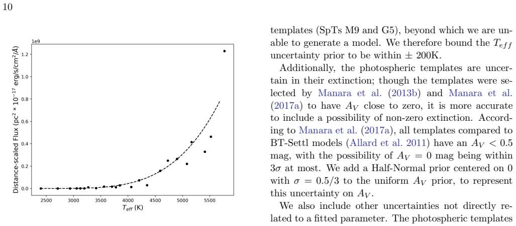
The load-bearing mechanism is a seven-parameter composite model of a YSO's blue-optical continuum: an isothermal hydrogen LTE slab (parameters Tslab, ne, tau0, and scaling Kslab) added to a scaled class III photospheric template (effective temperature Teff and scaling Kphot), then reddened by extinction AV. The argument is carried by the No-U-Turn Sampler, which explores the posterior over these parameters; to make Teff continuous, the code linearly interpolates between 23 observed class III templates whose fluxes and luminosities have been rescaled to follow a smooth polynomial relation. This machinery converts the previous discrete-grid chi-squared fitting approach into a full Bayesian inference that can report covariances and per-object uncertainty distributions for Lacc and Macc.
What would settle it
Take a set of YSOs with accretion luminosities measured independently from space-based ultraviolet spectra, fit the same VIRUS-resolution spectra with nuts-for-ysos, and check whether the posterior distributions for Lacc overlap the independent values: a systematic exclusion would show that the slab-model bolometric correction, the paper's load-bearing assumption, is biased.
Extended reading notes
Core claim
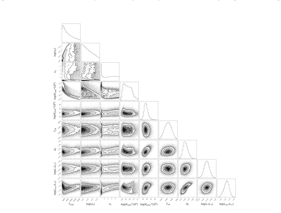
The central claim is that a Bayesian implementation of the standard continuum model can reliably recover the accretion luminosity and mass accretion rate of a young stellar object from a single low-resolution (R~800) optical spectrum, demonstrated on 15 YSOs observed with VIRUS. The method treats all seven model parameters as random variables and samples their joint posterior with the No-U-Turn Sampler, so that uncertainties in distance, extinction, template luminosity, spectral type, and the accretion model itself propagate into Lacc and Macc as full probability distributions. The derived values agree with emission-line-based accretion luminosities using the Alcalá et al. (2017) relations and occupy the same range as published results for Lupus, Chamaeleon I, and NGC1333. The authors further report that the slab parameters are largely nuisance parameters, that Lacc correlates strongly with extinction AV, and that five of the fifteen objects have accretion components consistent with zero and are therefore reported as upper limits.
Load-bearing premise
The results hinge on the assumption that integrating the isothermal hydrogen slab flux over 500-25000 Å gives the correct bolometric correction for the true accretion luminosity, even though the slab model is not physically tied to magnetospheric accretion.
Editorial extensions
If this is right
- With nuts-for-ysos, the same fitting procedure can be applied to spectra from other spectrographs by changing the spectral feature set; the authors demonstrate runs on HST STIS and X-Shooter spectra.
- Because the tool outputs posterior distributions for Lacc and Macc, future studies can quantify degeneracies such as the AV-Lacc correlation instead of quoting approximate 0.25 dex uncertainties.
- The method can identify weak accretors: five objects in the sample have slab components consistent with zero and are reported as upper limits, including two class II objects.
- Applied to larger VIRUS or other survey samples, the framework could populate the M*-Macc plane across many star-forming regions, which the authors argue is needed to understand the scatter in the mass-accretion relation.
Reading between the lines
- If the slab bolometric correction is biased, the emission-line check inherits the same bias because the Alcalá et al. (2017) Lline-Lacc relations were calibrated with the same slab method; an independent calibration would be required to break that circularity.
- The strong AV-Lacc correlation implies that for blue-limited, low-resolution spectra, extinction uncertainty sets a floor on how precisely any single-epoch accretion rate can be measured; adding longer-wavelength photometry should reduce it, which is a testable expectation.
- The same template-interpolation and posterior machinery could be transferred to other continuum-excess problems in YSO physics, such as veiling at higher resolution or near-infrared excesses, where similar degeneracies are present.
Signed reviews
Editorial analysis
A structured set of objections, weighed in public.
Referee Report
Summary. The paper presents nuts-for-ysos, a Bayesian (NUTS-based) framework that fits a simple isothermal LTE hydrogen-slab accretion model plus a class III photospheric template to low-resolution VIRUS spectra of 15 YSOs, simultaneously inferring Teff, AV, stellar luminosity, accretion luminosity, and mass accretion rate with full posterior uncertainties. The authors apply the code to archival VIRUS parallel observations, derive Lacc and Macc for the sample (with upper limits for five objects), and test the results against emission-line-based accretion luminosities using the Alcalá et al. (2017) Lline-Lacc relations and against literature values from Lupus, Chamaeleon I, and NGC 1333. The paper emphasizes that the Bayesian approach quantifies parameter covariances and uncertainties more completely than previous grid-based direct-method analyses, and it publicly releases the code and a Zenodo archive.
Significance. If the inferred accretion luminosities are reliable, the paper is a useful proof of concept: it demonstrates that a Bayesian sampler can be applied to the standard slab-plus-template continuum-fitting method, that the resulting posteriors expose degeneracies (notably AV-Lacc) that grid methods obscure, and that the tool can be transferred to other spectrographs. The public release of nuts-for-ysos and the explicit convergence checks (Rhat <= 1.1, thinning, posterior simulation) are strengths, as is the careful construction of the sample from HETVIPS data. The central limitation is that the verification is largely consistency testing rather than independent validation: the emission-line relations and most literature comparisons inherit the same slab-model bolometric correction, so a systematic bias in Lacc would propagate through the apparent agreement. The paper is honest about the slab model's lack of physical basis, but does not quantify the resulting systematic uncertainty in the final Macc values.
major comments (3)
- [Section 6 and Section 7.2] The validation is not independent of the fitting method. The Lline-Lacc relations from Alcalá et al. (2017) were calibrated using Lacc values obtained with the same slab-model continuum-fitting approach (Manara et al. 2013a), and the literature comparisons in Section 7.2 are dominated by studies that use the same direct slab method or, for Object 14, the Alcalá et al. (2017) relations. Thus the approximate 1:1 agreement in Figure 15 and the overlap in Figures 18 and 20 demonstrate self-consistency within the slab-model framework, not independent confirmation that the slab bolometric correction is correct. The paper should either add a genuinely independent test (e.g., shock-model-based Lacc estimates, or spectrally resolved Balmer-continuum studies) or explicitly reframe the claims of 'reliability' as consistency checks within the standard method.
- [Section 5.2 and Section 7.1] The derivation of Lacc integrates the slab flux over 500-25000 A, but the paper's own justification for the slab model is limited to agreement with shock models at wavelengths below about 3000 A, and the cited literature (Ingleby et al. 2013) shows that the slab and shock models diverge at longer wavelengths. If the bolometric correction from the isothermal LTE slab is biased over this full range, every Lacc and Macc in Tables 5 and 6 is biased in the same direction, and the emission-line and literature checks in Section 6 inherit that bias. The authors should quantify the sensitivity of Lacc to the integration range and to the choice of slab versus shock-model spectral shape, or present the bolometric-correction uncertainty as a dominant systematic term.
- [Section 4.3.1] The procedure of rescaling all photospheric template fluxes and luminosities so that their median fluxes follow a fourth-degree polynomial is an ad hoc renormalization that could affect the inferred Teff, Kphot, and hence Lstar and Mstar. The paper asserts that this 'does not fundamentally change the nature of the results' but provides no test of that assertion. Since Teff and Lstar feed into the mass and accretion-rate estimates via the evolutionary-track interpolation, the authors should demonstrate with a sensitivity analysis (e.g., fitting with and without the polynomial rescaling, or comparing against the original template grid) that the derived physical parameters are robust to this choice.
minor comments (4)
- [Section 6] The text states that the Alcalá et al. (2017) relations are 'completely independently derived' from the present data; this is true in the sense that they were calibrated on a different sample, but it is misleading because they were calibrated using the same slab-based direct method. Please rephrase to make the distinction between independence of data and dependence on the same accretion model clear.
- [Section 6, Object 12 discussion] The sentence 'the class III Object 12, which has Lacc,line = 0.36' appears to be missing a logarithm or a unit; presumably log(Lacc,line/Lsun) is meant. Please correct and ensure the value is shown with the same convention as in Table 5.
- [Table 5] For Objects 4 and 13, the table lists approximate values without uncertainties for several entries, while for other objects uncertainties are given. Please include a note or symbols indicating which quantities are approximate due to the Teff boundary issue, and consider providing the full posterior summaries for these objects in the appendix.
- [Section 4.3.2 and Section 5] The prior table lists the effective-temperature uncertainty as a bounded Normal distribution, but the text does not fully explain how this prior interacts with the template interpolation when Teff is near the grid edges. A sentence clarifying the behavior at the edges would help the reader assess the two boundary cases reported in Section 5.
Circularity Check
The central Bayesian Lacc fit is not circular, but the emission-line and literature verifications share the slab-model calibration used to build the comparison relations, so the validation is only partly independent.
-
fitted input called prediction
[Sections 4.1 and 6 (Alcalá et al. 2017 calibration description)]
"We use a slab of isothermal hydrogen in local thermodynamic equilibrium (LTE) ... This approach has been used numerous times in the past to derive accretion luminosities (e.g. ... Manara et al. (2013a); Alcalá et al. (2014, 2017)). ... Alcalá et al. (2017) studied X-shooter spectra of 81 class II or transition disk YSOs in Lupus, using the 'direct' method on each YSO by fitting the continuum model to each spectrum. They then updated empirical linear relationships between Lline and Lacc to calibrate the 'indirect' method."
The paper calls the emission-line check 'independently derived,' but the Alcalá et al. (2017) Lline-Lacc relations were calibrated against Lacc obtained with the same isothermal LTE slab 'direct' method that nuts-for-ysos uses. Applying those relations to VIRUS line luminosities therefore produces Lacc,line values that track slab-model Lacc by construction. A systematic error in the slab bolometric correction (e.g., from integrating the slab over 500-25000 Å when the model is justified mainly at <3000 Å) would appear on both sides of Figure 15, so the 1:1 agreement does not validate the model's absolute scale.
-
other
[Section 7.2, comparison with Lupus, Chamaeleon I, and NGC1333]
"With our small sample we can at least note that our results for the L∗-Lacc plot (Figure 8) and M∗-Macc plots (Figures 11 and 12) occupy a similar range as previous studies of various star-forming regions. ... Figure 18 shows that the L∗ and Lacc of our class II sample follow a loose linear relationship in agreement with these three star-forming regions."
The comparison values are not independent of the slab model: the Lupus (Alcalá et al. 2017) and Chamaeleon I (Manara et al. 2016) studies derive Lacc with the same direct slab-continuum method, and the NGC1333 comparison (Fiorellino et al. 2021) uses Pa-beta/Br-gamma relations from Alcalá et al. (2017), themselves slab-calibrated. Agreement with these samples therefore confirms consistency with earlier applications of the same model, but cannot detect a shared systematic bias in the slab bolometric correction.
1 more flagged steps
-
other
[Section 6, extinction correction of line fluxes]
"We correct the emission line fluxes for extinction using the AV derived from the continuum-fitting process in Section 4. We use the same AV so that the the direct and indirect methods can be consistently compared."
Both the continuum-derived Lacc and the line-derived Lacc,line are corrected with the same fitted AV posterior. If AV is biased, the two estimators shift together, so part of the Figure 15 agreement is inherited from this shared fitted input rather than from an independent measurement. This couples the two sides of the 'verification' without making the central fit definitional.
full rationale
The central derivation is not circular: nuts-for-ysos fits the slab plus photospheric template to continuum features (Section 4), then computes Lacc by integrating the fitted slab flux over 500-25000 Å (Section 5.2). That Lacc is a function of the fitted model, not an input, and the code was also tested for compatibility on HST ULYSSES and X-Shooter data. The circularity is confined to the validation layer. The paper explicitly describes the emission-line check as 'independently derived,' but the Alcalá et al. (2017) relations were calibrated on Lacc from the same isothermal LTE slab 'direct' method, and the paper itself notes the slab has no basis in the magnetospheric accretion picture (Sections 4.1 and 7.1). Consequently, the near-1:1 agreement in Figure 15 and the agreement with literature samples in Figures 18 and 20 are partly guaranteed by shared model assumptions and shared fitted AV, so they cannot validate the slab's bolometric correction. This is a real limitation of the verification, but the Bayesian estimation machinery, uncertainty propagation, and parameter-correlation results still have independent content. Score 4 (partial circularity in validation, not in the main derivation).
Assumptions & free parameters
free parameters (8)
- Tslab =
posterior, bounded 5000-11000 K
- ne =
posterior, bounded 1e10-1e16 cm-3
- tau0 =
posterior, bounded 0.01-5.0
- Kslab =
posterior, >0
- Kphot =
posterior, >0
- Teff =
posterior, bounded 2615-5550 K
- AV =
posterior, bounded 0-10 mag
- Fourth-degree polynomial for template flux rescaling =
coefficients from fit to 23 template median fluxes
assumptions (6)
- domain assumption Isothermal hydrogen LTE slab model represents the accretion excess continuum
- domain assumption Class III YSO spectra are valid photospheric templates for class II YSOs
- domain assumption Cardelli et al. (1989) reddening law with R_V=3.1 applies
- domain assumption Bailer-Jones et al. (2021) geometric distances with generalized gamma prior are correct
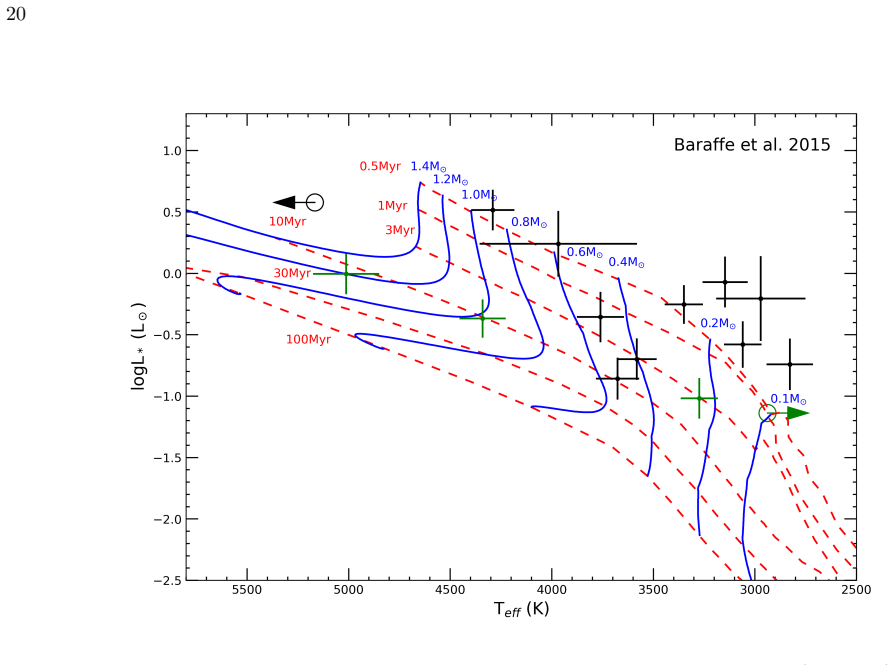
- domain assumption PMS evolutionary tracks (Baraffe+15, Siess+00) map Teff and L* to mass
- domain assumption Alcala et al. (2017) Lline-Lacc relations apply to these targets
Cite this review
Pith. "Pith review of A Bayesian Approach to Inferring Accretion Signatures in Young Stellar Objects: A Case Study with VIRUS." pith.science (2026). https://pith.science/paper/EGE7FFOB
@misc{pith2026250110500,
  author       = {Pith},
  title        = {Pith review of: A Bayesian Approach to Inferring Accretion Signatures in Young Stellar Objects: A Case Study with VIRUS},
  year         = {2026},
  howpublished = {\url{https://pith.science/paper/EGE7FFOB}},
  note         = {Machine review of arXiv:2501.10500}
}
abstract
The mass accretion rates of young stellar objects (YSOs) are key to understanding how stars form, how their circumstellar disks evolve, and even how planets form. We develop a Bayesian framework to determine the accretion rates of a sample of 15 YSOs using archival data from the VIRUS spectrograph ($R \sim 800$, 3500-5500\r{A}) on the Hobby-Eberly Telescope. We are publicly releasing our developed tool, dubbed nuts-for-ysos, as a Python package which can also be applied to other spectroscopic datasets. The nuts-for-ysos code fits a simple accretion model to the near-UV and optical continuum of each VIRUS spectrum. Our Bayesian approach aims to identify correlations between model parameters using the No U-Turn Sampler (NUTS). Moreover, this approach self-consistently incorporates all parameter uncertainties, allowing for a thorough estimation of the probability distribution for accretion rate not accomplished in previous works. Using nuts-for-ysos, we derive accretion rates of each YSO. We then verify the reliability of our method by comparing to results separately derived from only the spectral emission lines, and to results from earlier studies of the Lupus, Chamaeleon I, and NGC1333 regions. Finally, we discuss what qualitative trends, covariances, and degeneracies were found among model parameters. The technique developed in this paper is a useful improvement that can be applied in the future to larger samples of YSOs observed by VIRUS or other spectrographs.
Figures


Figures from the paper (46 more)






Reference graph
Works this paper leans on
-
[1]
, " * write output.state after.block = add.period write newline
ENTRY address archivePrefix author booktitle chapter doi edition editor eprint howpublished institution journal key month number organization pages publisher school series title misctitle type volume year version url label extra.label sort.label short.list INTEGERS output.state before.all mid.sentence after.sentence after.block FUNCTION init.state.consts ...
-
[2]
write newline
" write newline "" before.all 'output.state := FUNCTION format.url url empty "" new.block "" url * "" * if FUNCTION format.eprint eprint empty "" archivePrefix empty "" archivePrefix "arXiv" = new.block " " eprint * " " * new.block " " eprint * " " * if if if FUNCTION format.doi doi empty "" " " doi * " " * if FUNCTION format.pid doi empty eprint empty ur...
-
[3]
''TPv @Tvl1pxw G :(ڴi -ZڵkG㫯M6 K, ƴib֬Yy]HGrʾ d @!6l 'tRL6m? K.;.W^u5jԈ 5jDƍ O?=
thebibliography [1] 20pt to REFERENCES 6pt =0pt 10pt plus 3pt =0pt =0pt =1pt plus 1pt =0pt =0pt -12pt =13pt plus 1pt =20pt =13pt plus 1pt \@M =10000 =-1.0em =0pt =0pt 0pt =0pt =1.0em @enumiv\@empty 10000 10000 `\.\@m \@noitemerr \@latex@warning Empty `thebibliography' environment \@ifnextchar \@reference \@latexerr Missing key on reference command Each re...
2019
-
[4]
2019, arXiv e-prints, arXiv:1902.05569, 10.48550/arXiv.1902.05569
Akeson , R., Armus , L., Bachelet , E., et al. 2019, arXiv e-prints, arXiv:1902.05569, 10.48550/arXiv.1902.05569
-
[5]
2016, arXiv e-prints, abs/1605.02688
Al-Rfou, R., Alain, G., Almahairi, A., et al. 2016, arXiv e-prints, abs/1605.02688. http://arxiv.org/abs/1605.02688
arXiv 2016
-
[6]
Alcal \'a , J. M., Natta , A., Manara , C. F., et al. 2014, , 561, A2, 10.1051/0004-6361/201322254
-
[7]
Alcal \'a , J. M., Manara , C. F., Natta , A., et al. 2017, , 600, A20, 10.1051/0004-6361/201629929
-
[8]
2014, in Protostars and Planets VI, ed
Alexander , R., Pascucci , I., Andrews , S., Armitage , P., & Cieza , L. 2014, in Protostars and Planets VI, ed. H. Beuther , R. S. Klessen , C. P. Dullemond , & T. Henning , 475, 10.2458/azu_uapress_9780816531240-ch021
Show all 107 references
-
[9]
J., et al
Alexander , R., Rosotti , G., Armitage , P. J., et al. 2023, , 524, 3948, 10.1093/mnras/stad1983
2023 doi
-
[10]
2011, in Astronomical Society of the Pacific Conference Series, Vol
Allard , F., Homeier , D., & Freytag , B. 2011, in Astronomical Society of the Pacific Conference Series, Vol. 448, 16th Cambridge Workshop on Cool Stars, Stellar Systems, and the Sun, ed. C. Johns-Krull , M. K. Browning , & A. A. West , 91. 1011.5405
2011 arXiv
-
[11]
2014, , 572, A62, 10.1051/0004-6361/201423929
Antoniucci , S., Garc \' a L \'o pez , R., Nisini , B., et al. 2014, , 572, A62, 10.1051/0004-6361/201423929
2014 doi
-
[12]
P., Tollerud , E
Astropy Collaboration , Robitaille , T. P., Tollerud , E. J., et al. 2013, , 558, A33, 10.1051/0004-6361/201322068
2013 doi
-
[13]
M., Sip o cz , B
Astropy Collaboration , Price-Whelan , A. M., Sip o cz , B. M., et al. 2018, , 156, 123, 10.3847/1538-3881/aabc4f
2018 doi
-
[14]
M., Lim , P
Astropy Collaboration , Price-Whelan , A. M., Lim , P. L., et al. 2022, , 935, 167, 10.3847/1538-4357/ac7c74
2022 doi
-
[15]
2019, Specutils: Spectroscopic analysis and reduction , Astrophysics Source Code Library, record ascl:1902.012
Astropy-Specutils Development Team . 2019, Specutils: Spectroscopic analysis and reduction , Astrophysics Source Code Library, record ascl:1902.012. 1902.012
2019
-
[16]
Bailer-Jones , C. A. L., Rybizki , J., Fouesneau , M., Demleitner , M., & Andrae , R. 2021, , 161, 147, 10.3847/1538-3881/abd806
2021 doi
-
[17]
2015, , 577, A42, 10.1051/0004-6361/201425481
Baraffe , I., Homeier , D., Allard , F., & Chabrier , G. 2015, , 577, A42, 10.1051/0004-6361/201425481
2015 doi
-
[18]
M., Covino , E., et al
Biazzo , K., Alcal \'a , J. M., Covino , E., et al. 2012, , 547, A104, 10.1051/0004-6361/201219680
2012 doi
-
[19]
2020, C2D Candidate YSO STARS Catalog, IPAC, 10.26131/IRSA244
C2D Team . 2020, C2D Candidate YSO STARS Catalog, IPAC, 10.26131/IRSA244
2020 doi
-
[20]
1998, , 509, 802, 10.1086/306527
Calvet , N., & Gullbring , E. 1998, , 509, 802, 10.1086/306527
1998 doi
-
[21]
F., et al
Campbell-White , J., Sicilia-Aguilar , A., Manara , C. F., et al. 2021, , 507, 3331, 10.1093/mnras/stab2300
2021 doi
-
[22]
A., Clayton , G
Cardelli , J. A., Clayton , G. C., & Mathis , J. S. 1989, , 345, 245, 10.1086/167900
1989 doi
-
[23]
C., & Pan-STARRS Team
Chambers , K. C., & Pan-STARRS Team . 2017, in American Astronomical Society Meeting Abstracts, Vol. 229, American Astronomical Society Meeting Abstracts \#229, 223.03
2017
-
[24]
S., Hill , G
Chonis , T. S., Hill , G. J., Lee , H., et al. 2016, in Society of Photo-Optical Instrumentation Engineers (SPIE) Conference Series, Vol. 9908, Ground-based and Airborne Instrumentation for Astronomy VI, ed. C. J. Evans , L. Simard , & H. Takami , 99084C, 10.1117/12.2232209
2016 doi
-
[25]
Claes , R. A. B., Campbell-White , J., Manara , C. F., et al. 2024, , 690, A122, 10.1051/0004-6361/202450885
2024 doi
-
[26]
J., & Pringle , J
Clarke , C. J., & Pringle , J. E. 2006, , 370, L10, 10.1111/j.1745-3933.2006.00177.x
2006
-
[27]
2021, , 647, A116, 10.1051/0004-6361/202038516
Cornu , D., & Montillaud , J. 2021, , 647, A116, 10.1051/0004-6361/202038516
2021 doi
-
[28]
M., Wright , E
Cutri , R. M., Wright , E. L., Conrow , T., et al. 2021, VizieR Online Data Catalog, II/328
2021
-
[29]
P., Natta , A., & Testi , L
Dullemond , C. P., Natta , A., & Testi , L. 2006, , 645, L69, 10.1086/505744
2006 doi
-
[30]
2020, Gaia EDR3, European Space Agency, 10.5270/esa-1ugzkg7
EDR3, G. 2020, Gaia EDR3, European Space Agency, 10.5270/esa-1ugzkg7
2020 doi
-
[31]
E., Rosotti , G., & Manara , C
Ercolano , B., Mayr , D., Owen , J. E., Rosotti , G., & Manara , C. F. 2014, , 439, 256, 10.1093/mnras/stt2405
2014 doi
-
[32]
C., Herczeg , G
Espaillat , C. C., Herczeg , G. J., Thanathibodee , T., et al. 2022, , 163, 114, 10.3847/1538-3881/ac479d
2022 doi
-
[33]
E., Blake , G
Evans , Neal J., I., Allen , L. E., Blake , G. A., et al. 2003, , 115, 965, 10.1086/376697
2003 doi
-
[34]
2023, , 944, 135, 10.3847/1538-4357/aca320
Fiorellino , E., Tychoniec , ., Cruz-S \'a enz de Miera , F., et al. 2023, , 944, 135, 10.3847/1538-4357/aca320
2023 doi
-
[35]
F., Nisini , B., et al
Fiorellino , E., Manara , C. F., Nisini , B., et al. 2021, , 650, A43, 10.1051/0004-6361/202039264
2021 doi
-
[36]
Gaia Collaboration , Prusti , T., de Bruijne , J. H. J., et al. 2016, , 595, A1, 10.1051/0004-6361/201629272
2016 doi
-
[37]
Gaia Collaboration , Brown , A. G. A., Vallenari , A., et al. 2018, , 616, A1, 10.1051/0004-6361/201833051
2018 doi
-
[38]
2021, , 649, A1, 10.1051/0004-6361/202039657
---. 2021, , 649, A1, 10.1051/0004-6361/202039657
2021 doi
-
[39]
2018, Gaia DR2, European Space Agency, 10.5270/esa-ycsawu7
Gaia DR2 . 2018, Gaia DR2, European Space Agency, 10.5270/esa-ycsawu7
2018 doi
-
[40]
2012, in American Astronomical Society Meeting Abstracts, Vol
Gebhardt , K., Hill , G., Komatsu , E., et al. 2012, in American Astronomical Society Meeting Abstracts, Vol. 219, American Astronomical Society Meeting Abstracts \#219, 424.02
2012
-
[41]
2021, , 923, 217, 10.3847/1538-4357/ac2e03
Gebhardt , K., Mentuch Cooper , E., Ciardullo , R., et al. 2021, , 923, 217, 10.3847/1538-4357/ac2e03
2021 doi
-
[42]
Gelman , A., & Rubin , D. B. 1992, Statistical Science, 7, 457, 10.1214/ss/1177011136
1992
-
[43]
2011, PySpecKit: Python Spectroscopic Toolkit , Astrophysics Source Code Library, record ascl:1109.001
Ginsburg , A., & Mirocha , J. 2011, PySpecKit: Python Spectroscopic Toolkit , Astrophysics Source Code Library, record ascl:1109.001. 1109.001
2011
-
[44]
P., Wilking , B
Greene , T. P., Wilking , B. A., Andre , P., Young , E. T., & Lada , C. J. 1994, , 434, 614, 10.1086/174763
1994 doi
-
[45]
2000, , 544, 927, 10.1086/317253
Gullbring , E., Calvet , N., Muzerolle , J., & Hartmann , L. 2000, , 544, 927, 10.1086/317253
2000 doi
-
[46]
1998, , 492, 323, 10.1086/305032
Gullbring , E., Hartmann , L., Brice \ n o , C., & Calvet , N. 1998, , 492, 323, 10.1086/305032
1998 doi
-
[47]
R., Millman, K
Harris, C. R., Millman, K. J., van der Walt, S. J., et al. 2020, Nature, 585, 357, 10.1038/s41586-020-2649-2
2020 doi
-
[48]
1998, , 495, 385, 10.1086/305277
Hartmann , L., Calvet , N., Gullbring , E., & D'Alessio , P. 1998, , 495, 385, 10.1086/305277
1998 doi
-
[49]
2016, , 54, 135, 10.1146/annurev-astro-081915-023347
Hartmann , L., Herczeg , G., & Calvet , N. 2016, , 54, 135, 10.1146/annurev-astro-081915-023347
2016 doi
-
[50]
M., Huard , T
Harvey , P. M., Huard , T. L., J rgensen , J. K., et al. 2008, , 680, 495, 10.1086/587687
2008 doi
-
[51]
J., & Hillenbrand , L
Herczeg , G. J., & Hillenbrand , L. A. 2008, , 681, 594, 10.1086/586728
2008 doi
-
[52]
2014, , 786, 97, 10.1088/0004-637X/786/2/97
---. 2014, , 786, 97, 10.1088/0004-637X/786/2/97
2014 doi
-
[53]
J., Kelz , A., Lee , H., et al
Hill , G. J., Kelz , A., Lee , H., et al. 2018, in Society of Photo-Optical Instrumentation Engineers (SPIE) Conference Series, Vol. 10702, Ground-based and Airborne Instrumentation for Astronomy VII, ed. C. J. Evans , L. Simard , & H. Takami , 107021K, 10.1117/12.2314280
2018 doi
-
[54]
J., Lee , H., MacQueen , P
Hill , G. J., Lee , H., MacQueen , P. J., et al. 2021, , 162, 298, 10.3847/1538-3881/ac2c02
2021 doi
-
[55]
D., & Gelman, A
Hoffman, M. D., & Gelman, A. 2014, J. Mach. Learn. Res., 15, 1593
2014
-
[56]
Hunter, J. D. 2007, Computing in Science & Engineering, 9, 90, 10.1109/MCSE.2007.55
2007 doi
-
[57]
2013, , 767, 112, 10.1088/0004-637X/767/2/112
Ingleby , L., Calvet , N., Herczeg , G., et al. 2013, , 767, 112, 10.1088/0004-637X/767/2/112
2013 doi
-
[58]
M., Grupp , F., et al
Kelz , A., Bauer , S. M., Grupp , F., et al. 2006, in Society of Photo-Optical Instrumentation Engineers (SPIE) Conference Series, Vol. 6273, Society of Photo-Optical Instrumentation Engineers (SPIE) Conference Series, ed. E. Atad-Ettedgui , J. Antebi , & D. Lemke , 62733W, 10...
2006 doi
- [59]
-
[60]
P., & Leisawitz , D
Koenig , X. P., & Leisawitz , D. T. 2014, , 791, 131, 10.1088/0004-637X/791/2/131
2014 doi
- [61]
-
[62]
L., Stauffer , J
Luhman , K. L., Stauffer , J. R., Muench , A. A., et al. 2003, , 593, 1093, 10.1086/376594
2003 doi
-
[63]
Lynden-Bell , D., & Pringle , J. E. 1974, , 168, 603, 10.1093/mnras/168.3.603
1974 doi
-
[64]
2012, in Society of Photo-Optical Instrumentation Engineers (SPIE) Conference Series, Vol
Mahadevan , S., Ramsey , L., Bender , C., et al. 2012, in Society of Photo-Optical Instrumentation Engineers (SPIE) Conference Series, Vol. 8446, Ground-based and Airborne Instrumentation for Astronomy IV, ed. I. S. McLean , S. K. Ramsay , & H. Takami , 84461S, 10.1117/12.926102
2012 doi
-
[65]
W., Terrien , R., et al
Mahadevan , S., Ramsey , L. W., Terrien , R., et al. 2014, in Society of Photo-Optical Instrumentation Engineers (SPIE) Conference Series, Vol. 9147, Ground-based and Airborne Instrumentation for Astronomy V, ed. S. K. Ramsay , I. S. McLean , & H. Takami , 91471G, 10.1117/12.2056417
2014 doi
-
[66]
Manara , C. F. 2014, PhD thesis, Ludwig-Maximilans-Universitat Munchen
2014
-
[67]
Manara , C. F. 2018, in Protoplanetary Disks Seen through the Eyes of New-Generation High-Resolution Instruments, 23, 10.5281/zenodo.1892514
2018 doi
-
[68]
F., Ansdell , M., Rosotti , G
Manara , C. F., Ansdell , M., Rosotti , G. P., et al. 2023, in Astronomical Society of the Pacific Conference Series, Vol. 534, Astronomical Society of the Pacific Conference Series, ed. S. Inutsuka , Y. Aikawa , T. Muto , K. Tomida , & M. Tamura , 539, 10.48550/arXiv.2203.09930
-
[69]
F., Beccari , G., Da Rio , N., et al
Manara , C. F., Beccari , G., Da Rio , N., et al. 2013 a , , 558, A114, 10.1051/0004-6361/201321866
2013 doi
-
[70]
F., Fedele , D., Herczeg , G
Manara , C. F., Fedele , D., Herczeg , G. J., & Teixeira , P. S. 2016, , 585, A136, 10.1051/0004-6361/201527224
2016 doi
-
[71]
F., Frasca , A., Alcal \'a , J
Manara , C. F., Frasca , A., Alcal \'a , J. M., et al. 2017 a , , 605, A86, 10.1051/0004-6361/201730807
2017 doi
-
[72]
F., Mordasini , C., Testi , L., et al
Manara , C. F., Mordasini , C., Testi , L., et al. 2019, , 631, L2, 10.1051/0004-6361/201936488
2019 doi
-
[73]
F., Testi , L., Rigliaco , E., et al
Manara , C. F., Testi , L., Rigliaco , E., et al. 2013 b , , 551, A107, 10.1051/0004-6361/201220921
2013 doi
-
[74]
F., Testi , L., Herczeg , G
Manara , C. F., Testi , L., Herczeg , G. J., et al. 2017 b , , 604, A127, 10.1051/0004-6361/201630147
2017 doi
-
[75]
F., Natta , A., Rosotti , G
Manara , C. F., Natta , A., Rosotti , G. P., et al. 2020, , 639, A58, 10.1051/0004-6361/202037949
2020 doi
-
[76]
2020, , 893, 56, 10.3847/1538-4357/ab7ead
Manzo-Mart \' nez , E., Calvet , N., Hern \'a ndez , J., et al. 2020, , 893, 56, 10.3847/1538-4357/ab7ead
2020 doi
- [77]
-
[78]
2019, , 487, 2522, 10.1093/mnras/stz1301
Marton , G., \'A brah \'a m , P., Szegedi-Elek , E., et al. 2019, , 487, 2522, 10.1093/mnras/stz1301
2019 doi
-
[79]
Meng , H. Y. A., Rieke , G. H., Su , K. Y. L., & G \'a sp \'a r , A. 2017, , 836, 34, 10.3847/1538-4357/836/1/34
2017 doi
-
[80]
1998, , 492, 743, 10.1086/305069
Muzerolle , J., Calvet , N., & Hartmann , L. 1998, , 492, 743, 10.1086/305069
1998 doi
-
[81]
L., Brice \ n o , C., Hartmann , L., & Calvet , N
Muzerolle , J., Luhman , K. L., Brice \ n o , C., Hartmann , L., & Calvet , N. 2005, , 625, 906, 10.1086/429483
2005 doi
-
[82]
2004, , 424, 603, 10.1051/0004-6361:20040356
Natta , A., Testi , L., Muzerolle , J., et al. 2004, , 424, 603, 10.1051/0004-6361:20040356
2004 doi
-
[83]
2006, , 452, 245, 10.1051/0004-6361:20054706
Natta , A., Testi , L., & Randich , S. 2006, , 452, 245, 10.1051/0004-6361:20054706
2006 doi
-
[84]
2000, , 143, 23, 10.1051/aas:2000169
Ochsenbein , F., Bauer , P., & Marcout , J. 2000, , 143, 23, 10.1051/aas:2000169
2000 doi
-
[85]
V., Espaillat , C
Pittman , C. V., Espaillat , C. C., Robinson , C. E., et al. 2022, , 164, 201, 10.3847/1538-3881/ac898d
2022 doi
-
[86]
Planck Collaboration , Adam , R., Ade , P. A. R., et al. 2016, , 594, A10, 10.1051/0004-6361/201525967
2016 doi
-
[87]
2023, PyTensor, GitHub
PyMC Team . 2023, PyTensor, GitHub. https://github.com/pymc-devs/pytensor
2023
-
[88]
W., Adams , M
Ramsey , L. W., Adams , M. T., Barnes , T. G., et al. 1998, in Society of Photo-Optical Instrumentation Engineers (SPIE) Conference Series, Vol. 3352, Advanced Technology Optical/IR Telescopes VI, ed. L. M. Stepp , 34--42, 10.1117/12.319287
1998 doi
-
[89]
M., Guieu , S., Stauffer , J
Rebull , L. M., Guieu , S., Stauffer , J. R., et al. 2011, , 193, 25, 10.1088/0067-0049/193/2/25
2011 doi
-
[90]
2012, , 548, A56, 10.1051/0004-6361/201219832
Rigliaco , E., Natta , A., Testi , L., et al. 2012, , 548, A56, 10.1051/0004-6361/201219832
2012 doi
-
[91]
R., Taylor , J
Roman-Duval , J., Proffitt , C. R., Taylor , J. M., et al. 2020, Research Notes of the American Astronomical Society, 4, 205, 10.3847/2515-5172/abca2f
2020 doi
-
[92]
2018, , 609, A70, 10.1051/0004-6361/201630111
Rugel , M., Fedele , D., & Herczeg , G. 2018, , 609, A70, 10.1051/0004-6361/201630111
2018 doi
-
[93]
V., & Fonnesbeck , C
Salvatier , J., Wiecki , T. V., & Fonnesbeck , C. 2016, PeerJ Computer Science, 10.7717/peerj-cs.55
2016 doi
-
[94]
1994, , 429, 781, 10.1086/174363
Shu , F., Najita , J., Ostriker , E., et al. 1994, , 429, 781, 10.1086/174363
1994 doi
-
[95]
2000, , 358, 593
Siess , L., Dufour , E., & Forestini , M. 2000, , 358, 593. astro-ph/0003477
2000 arXiv
- [96]
-
[97]
2022, Pan-STARRS1 DR2 Catalog, STScI/MAST, 10.17909/S0ZG-JX37
STScI . 2022, Pan-STARRS1 DR2 Catalog, STScI/MAST, 10.17909/S0ZG-JX37
2022 doi
-
[98]
1985, , 37, 515
Uchida , Y., & Shibata , K. 1985, , 37, 515
1985
-
[99]
A., Basri , G., & Johns , C
Valenti , J. A., Basri , G., & Johns , C. M. 1993, , 106, 2024, 10.1086/116783
1993 doi
-
[100]
Van Rossum, G., & Drake, F. L. 2009, Introduction to python 3: python documentation manual part 1 (CreateSpace)
2009
-
[101]
M., et al
Venuti , L., Stelzer , B., Alcal \'a , J. M., et al. 2019, , 632, A46, 10.1051/0004-6361/201935745
2019 doi
-
[102]
2011, , 536, A105, 10.1051/0004-6361/201117752
Vernet , J., Dekker , H., D'Odorico , S., et al. 2011, , 536, A105, 10.1051/0004-6361/201117752
2011 doi
-
[103]
E., et al
Virtanen, P., Gommers, R., Oliphant, T. E., et al. 2020, Nature Methods, 17, 261, 10.1038/s41592-019-0686-2
2020 doi
- [104]
-
[105]
A Bayesian Approach to Inferring Accretion Signatures in Young Stellar Objects: A Case Study with VIRUS
Willett, L. H., Ninan, J., Mahadevan, S., et al. 2024, nuts-for-ysos v1.1: Software used in "A Bayesian Approach to Inferring Accretion Signatures in Young Stellar Objects: A Case Study with VIRUS", Zenodo, 10.5281/ZENODO.13955222
2024 doi
-
[106]
2019, AllWISE Source Catalog, IPAC, 10.26131/IRSA1
WISE . 2019, AllWISE Source Catalog, IPAC, 10.26131/IRSA1
2019 doi
-
[107]
R., Debski , M
Zeimann , G. R., Debski , M. H., Schneider , D. P., et al. 2024, , 966, 14, 10.3847/1538-4357/ad35b8
2024 doi
Reviewed August 10, 2026 · model on record in the stance chip above.
Discussion (0). Continue with ORCID to comment.