REVIEW 3 major objections 6 minor 84 references
Detection of Unresolved Strongly Lensed Supernovae with 7-Dimensional Telescope
T0 review · 3 major / 6 minor · reviewed 2026-08-10 · deepseek-v4-flash
Pith's one-line read The authors forecast that the 7-Dimensional Telescope, an array of twenty 50-cm telescopes, can detect about 7 Type Ia and 9 core-collapse lensed supernovae per year in known lens fields, and that follow-up of a subset could measure the…
desk verdict A useful, honest forecast of how a small-telescope array could find unresolved lensed SNe; the order-of-magnitude rates are plausible, but the specific numbers and the H0 forecast rest on assumptions a referee should probe. read the letter →
The pith
A machine-rendered reading of the paper's core claim, the machinery that carries it, and where it could break.
The reading
What carries the argument
The detection forecast is carried by synthetic light curves: SNCosmo with the SALT3 model for Type Ia and six template families for core-collapse subtypes, with image multiplicities, log-normal magnifications, and exponential time delays (mean 6.83 days) tuned to the unresolved, short-delay population inferred from ZTF and LSST studies, and with a system counted as detected when the combined (unresolved) light curve rises above the survey depth for a control time long enough to be caught. The cosmological forecast is carried by the time-delay distance relation $H_0 D_{\Delta t} = (1+z_l)\, H_0 D_l\, H_0 D_s / H_0 D_{ls}$, evaluated with distances from Gaussian-process reconstructions of the unanchored luminosity distance $H_0 D_L(z)$ built from the Pantheon sample, and then compared against mock time-delay distances drawn from a flat $\Lambda$CDM fiducial model with 10% noise; $H_0$ is obtained by marginalizing over the Gaussian-process realizations.
What would settle it
Count the number of the 5,807 candidate lens fields that contain a bright background source at $z_s \lesssim 0.7$ using existing deep imaging; the predicted annual yields are nearly proportional to that count, so a much smaller population would collapse the forecast. A direct empirical check is the first year of the proposed 7DT $r$-band monitoring: observing far fewer than roughly 17 unresolved lensed supernovae would indicate that the source-redshift tail, the magnification distribution, or the unresolved fraction is more optimistic than reality.
Extended reading notes
Core claim
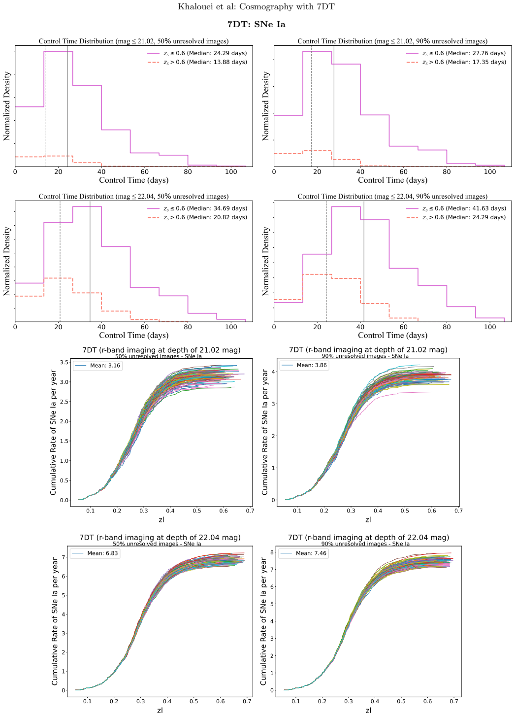
The central claim is that unresolved, blended gravitationally lensed supernovae are detectable at useful rates with a small-aperture multi-telescope system, and that the systems thereby found are sufficient for a model-independent constraint on the Hubble constant. Under ideal conditions, monitoring the strong-lens and candidate sample in the $r$-band at a depth of 22.04 mag yields maximum annual rates of 7.46 Type Ia and 9.49 core-collapse detections, split among the core-collapse subtypes (2.49 Ic, 0.80 IIb, 0.52 IIL, 0.78 IIn, 3.75 IIP, 1.15 Ib); a shallower medium-band program at 20.61 mag yields 2.53 Type Ia events per year. Taking the detected systems as the input to a model-independent Gaussian-process analysis that anchors the Pantheon supernova distances to measured time-delay distances, the forecast returns $H_0 = 70.03 \pm 1.9$ km/s/Mpc, i.e., 2.7% precision, for a combined sample of seven Type Ia and seven core-collapse systems.
Load-bearing premise
The entire detection-rate forecast rests on the assumed redshift distribution of the supernova sources behind the lens candidates, specifically the low-redshift tail below $z_s = 0.7$ that the 7DT can actually see; the paper imposes this tail by multiplying the lens redshift distribution with a truncated normal distribution rather than measuring it from the lens catalog or from observed lensed supernovae.
Editorial extensions
If this is right
- Under ideal conditions, the 7DT target program in the $r$-band at depth 22.04 mag should detect about 7.46 Type Ia and 9.49 core-collapse lensed supernovae per year within the ~1,125 fields covering 5,807 strong-lens systems and candidates.
- The 7DS wide-field medium-band program at the m6000 filter depth of 20.61 mag is forecast to detect about 2.53 Type Ia lensed supernovae per year.
- Following up seven Type Ia and seven core-collapse detections with larger telescopes, the model-independent Gaussian-process method yields $H_0 = 70.03 \pm 1.9$ km/s/Mpc, a 2.7% precision measurement.
- Unresolved glSNe, having median time delays of a few days, are the bright, blended channel that small telescopes can catch; the trade-off is that short delays worsen time-delay-measurement precision for $H_0$.
- A complementary strategy, proposed but not simulated, places 7DT monitoring in LSST's low-cadence rolling-season fields to add early detection and medium-band classification where LSST coverage is sparse.
Reading between the lines
- The yield is calibratable before the survey runs: a count of $z_s \lesssim 0.7$ background sources behind the candidate fields, from existing deep multi-band imaging, would pin down the dominant uncertainty in the rate forecast.
- The 2.7% $H_0$ precision should be read as an ideal-case bound rather than a guaranteed outcome, since the simulated systems have short delays and the paper itself flags these as disadvantaged for precise time-delay measurement; including microlensing, which the paper sets aside, would tend to add scatter on exactly these short-delay systems.
- The same control-time machinery transfers to other small-telescope arrays and to larger future lens catalogs, so the reusable result is the method for turning an unresolved-transient survey into a lensed-supernova yield estimate, not just the 7DT numbers.
Editorial analysis
A structured set of objections, weighed in public.
Referee Report
Summary. The paper simulates the detection of unresolved strongly lensed supernovae with the 7DT small-telescope array, using 5807 strong lens candidates from DECaLS/DESI Legacy Surveys. It predicts annual detection rates for Type Ia and several core-collapse subtypes under different 7DT observing strategies, and uses a Gaussian-process, model-independent method with Pantheon SNe Ia to forecast H0 precision from follow-up of the detected systems. The headline results are 7.46 SNe Ia yr^-1 and 9.49 CC SNe yr^-1 (sum of subtypes) in the r-band deep target mode at 22.04 mag, and 2.53 SNe Ia yr^-1 in the WTS medium-band program, leading to a forecasted 2.7% H0 precision (70.03 ± 1.9 km/s/Mpc) from 7 Ia + 7 CC systems.
Significance. If the rates and H0 precision hold, this would demonstrate that a modest-aperture, wide-field telescope array can contribute to glSNe discovery and time-delay cosmography, complementing LSST and Roman. The paper includes a concrete simulation pipeline, explicit SN-rate formulas imported from the literature, and a reproducible GP-based analysis framework. The main value is in showing the feasibility of unresolved glSNe detection with small telescopes; however, the quantitative forecasts are currently undermined by inconsistencies in the source-redshift prescription and an unsupported time-delay distance uncertainty assumption.
major comments (3)
- [Section 3.1] The source-redshift prescription as written is internally inconsistent: a truncated normal N(2,0.5) with lower bound 1 has zero probability below zs=0.7, yet the text immediately applies a selection zs < 0.7, and Figures 3, 5, and 6 show simulated source redshifts below 0.7. Taken literally, the simulation would produce no systems at all, while the paper reports nonzero rates (e.g., 7.46 SNe Ia yr^-1 and the 7 Ia + 7 CC sample used in Section 4). Please correct the description (e.g., if the implementation is zs = zl × x with x drawn from a truncated normal, state that explicitly) or re-run the simulation with the stated distribution and re-derive the rates. As written, the central detection-rate and H0-precision forecasts are not reproducible.
- [Section 4, Eq. (4)] The H0 forecast assumes sigma_DDelta_t = 0.1 D for every mock system, including unresolved systems whose simulated time delays have a median of 6.83 days (Section 3.3). The paper itself notes that short delays are disadvantaged for precise time-delay measurements. A 10% time-delay distance uncertainty for a few-day delay in an unresolved, blended system is optimistic and is the main driver of the 2.7% precision in Table 2. Please justify this assumption with a realistic error budget or present the H0 precision as a function of sigma_DDelta_t; otherwise the forecast is a self-consistency check of the assumed noise rather than a prediction of the 7DT+follow-up program.
- [Sections 3.1 and 3.4] The headline detection rates are quoted as 'maximum expected' under ideal conditions, but the simulation uses the full 5807-candidate sample without a lens-likelihood threshold (Figure 2 shows many candidates with likelihood near 0.1–0.3), assumes 100% observing efficiency and 7-hour nights with no weather or moon-phase losses, and does not model the lens-galaxy subtraction or image blending in detail. Please provide a fiducial scenario (e.g., applying a likelihood cut, adopting a weather fraction, or including a detection-efficiency factor) alongside the ideal-case maxima, so that the annual rates quoted in the abstract are not read as realistic expectations.
minor comments (6)
- [Section 3.3] Change 'microlensig' to 'microlensing'.
- [Section 3.1] Clarify the relation between the 5807-candidate parent sample and the ~1225 systems within the 7DT footprint; the text says 'around 1225 lens systems and candidates' but does not state the declination or likelihood cuts used.
- [Abstract and Table 1] Unify the WTS depth: the abstract quotes 20.61 mag for the m6000 filter, while Table 1 lists 20.60 for m600; also the filter is referred to as both m6000 and m600.
- [Figure 5 caption] The caption states zs <= 0.6, while Section 3.4.1 says systems with 0.6 < zs < 0.7 are not detectable; make the redshift ranges consistent across text and figures.
- [Section 4] Equation (3) uses H0DDelta_t but does not define DDelta_t before first use; add a sentence defining the time-delay distance.
- [Throughout] Fix rendering artifacts in author names (e.g., 'Sagu´ es', 'Ca˜ nameras') and the spacing in '2 .7%' in the abstract.
Circularity Check
Detection-rate simulation is self-contained; the quoted 2.7% H0 precision reduces to the assumed 10% time-delay-distance noise divided by sqrt(14).
-
fitted input called prediction
[Section 4 (Eq. 4 and Table 2)]
"This mock data is calculated by taking a flat ΛCDM model with H0 = 70 km/s/Mpc and Ωm = 0.3 ... Then 10% noise is added to these mock time-delay distances, which we estimate to be a reasonable uncertainty associated with the time-delay distances (σD∆t,i = 0.1Dsim∆t,i). ... Table 2 ... 7 Ia + 7 CC (Broad-band) 70.03 ± 1.9 2.7%"
The forecast precision is not an output of the survey simulation or the Gaussian-process machinery; it is the input per-system fractional uncertainty divided by the square root of the number of systems. With σ_DΔt/D = 10% and N = 14, 10%/√14 = 2.7%, exactly the Table 2 value (and 10%/√7 = 3.8% for the 7-Ia row). Because the mock DΔt are generated from the same H0 = 70 fiducial model used in the likelihood, the recovered central value 70.03 is enforced by construction. The '2.7% precision' is therefore a restatement of the assumed noise and chosen sample size, not an independent prediction derived from 7DT's detection capability.
full rationale
The detection-rate simulation is self-contained: rates are computed by Monte Carlo over the selected DECaLS lens catalog with imported SN-rate formulas (Shu et al. 2018), SALT3/Nugent light-curve models, and explicitly stated magnification and time-delay distributions; the quoted yields (7.46 Ia, etc.) do not reduce to any fitted quantity. The source-redshift recipe in §3.1 (lens distribution multiplied by a truncated normal with lower bound 1, then selecting zs < 0.7) is a modeling prior imported from Sheu et al. 2023, not a circular step; it is an assumption that controls the yield and deserves external calibration, but that is a robustness/correctness concern rather than circularity. Several citations (Liao et al. 2019, 2020; Bag et al. 2021, 2024; Sheu et al. 2023) include the present authors, but the methods are re-implemented in the text rather than invoked as black-box theorems, so the self-citations are not load-bearing. The one genuine reduction is in the H0 forecast: the quoted 2.7% precision for 7 Ia + 7 CC equals 10%/√14, i.e., the assumed per-system time-delay-distance uncertainty divided by the square root of the sample size, and the recovered central value is forced by generating the mock data from H0 = 70. This makes the cosmological precision forecast a statistically forced restatement of its input assumptions. The circularity is partial and localized to the cosmological forecast, not to the detection-rate simulation, hence a score of 4.
Assumptions & free parameters
free parameters (6)
- Source redshift distribution of lensed SNe =
N(2,0.5), truncated at lower bound 1; selection cut z_s < 0.7
- Unresolved image magnification distribution =
log-normal with mean 1.07 and std 0.465 (converted from Sagues Carracedo et al. 2024)
- Unresolved time-delay distribution =
exponential with mean 6.83 days
- Time-delay distance fractional uncertainty =
10% (sigma_Ddt = 0.1 D_sim)
- Fraction of systems with completely unresolved images =
50% or 90% (scenarios)
- Host galaxy dust extinction parameters =
E(B-V)_host up to 0.2, R_V in [1.63, 3.85]
assumptions (6)
- domain assumption Lensed SN rates follow cosmic star formation history (kcc=0.0068 per solar mass; SNe Ia delay-time distribution t_D^-1.07)
- domain assumption The DECaLS strong-lens candidate catalog used here (Huang et al. 2020, 2021; Storfer et al. 2024) is representative of real lens systems and is used without a lens-probability cut
- domain assumption Unresolved lensed SN light curves can be modeled as the simple sum of 2 or 4 image fluxes with no microlensing
- standard math Gaussian process reconstruction of H0D_L from Pantheon SNe Ia, anchored by time-delay distances, recovers H0 without model bias
- domain assumption Mock time-delay distances are generated from flat LambdaCDM with H0=70 km/s/Mpc and Omega_m=0.3, then 10% noise is added
- ad hoc to paper Source redshifts are drawn by multiplying the lens redshift distribution by a truncated normal N(2,0.5) with lower bound 1, then cutting at z_s<0.7
Cite this review
Pith. "Pith review of Detection of Unresolved Strongly Lensed Supernovae with 7-Dimensional Telescope." pith.science (2026). https://pith.science/paper/GKQNZDH3
@misc{pith2026250112525,
  author       = {Pith},
  title        = {Pith review of: Detection of Unresolved Strongly Lensed Supernovae with 7-Dimensional Telescope},
  year         = {2026},
  howpublished = {\url{https://pith.science/paper/GKQNZDH3}},
  note         = {Machine review of arXiv:2501.12525}
}
abstract
Gravitationally lensed supernovae (glSNe) are a powerful tool for exploring the realms of astronomy and cosmology. Time-delay measurements and lens modeling of glSNe can provide a robust and independent method for constraining the expansion rate of the universe. The study of unresolved glSNe light curves presents a unique opportunity for utilizing small telescopes to investigate these systems. In this work, we investigate diverse observational strategies for the initial detection of glSNe using the 7-Dimensional Telescope (7DT), a multitelescope system composed of twenty 50-cm telescopes. We implement different observing strategies on a subset of 5807 strong lensing systems and candidates identified within the Dark Energy Camera Legacy Survey (DECaLS), as reported in various publications. Our simulations under ideal observing conditions indicate the maximum expected annual detection rates for various glSNe types (Type Ia and core-collapse (CC)) using the 7DT target observing mode in the $r$-band at a depth of 22.04 mag, as follows: 7.46 events for type Ia, 2.49 for type Ic, 0.8 for type IIb, 0.52 for type IIL, 0.78 for type IIn, 3.75 for type IIP, and 1.15 for type Ib. Furthermore, in the case of medium-band filter observations (m6000) at a depth of 20.61 in the Wide-field Time-domain Survey (WTS)program, the predicted detection rate for glSNe Ia is 2.53 $yr^{-1}$. Given targeted follow-up observations of these initially detected systems with more powerful telescopes, we can apply a model-independent approach to forecast the ability to measure $H_{0}$ using a Gaussian process from Type Ia Supernovae (SNe Ia) data and time-delay distance information derived from glSNe systems, which include both Ia and CC types. We forecast that the expected detection rate of glSNe systems can achieve a $2.7\%$ precision in estimating the $H_{0}$.
Figures


Figures from the paper (4 more)



Reference graph
Works this paper leans on
-
[1]
2021, MNRAS, 504, 4667
Alam, S., de Mattia, A., Tamone, A., et al. 2021, MNRAS, 504, 4667
2021
-
[2]
2024, MNRAS, 531, 3509
Arendse, N., Dhawan, S., Sagu´ es Carracedo, A., et al. 2024, MNRAS, 531, 3509
2024
-
[3]
H., et al
Bag, S., Huber, S., Suyu, S. H., et al. 2024, A&A, 691, A100
2024
-
[4]
G., Linder, E
Bag, S., Kim, A. G., Linder, E. V., & Shafieloo, A. 2021, ApJ, 910, 65
2021
-
[5]
2024, Zenodo, doi: https://zenodo.org/records/10602402
Barbary, K., Bailey, S., Barentsen, G., et al. 2024, Zenodo, doi: https://zenodo.org/records/10602402
- [6]
-
[7]
Birrer, S., Dhawan, S., & Shajib, A. J. 2022, ApJ, 924, 2
work page 2022
-
[8]
J., Galan, A., et al
Birrer, S., Shajib, A. J., Galan, A., et al. 2020, A&A, 643, A165
2020
Show all 84 references
-
[9]
& Treu, T
Birrer, S. & Treu, T. 2021, A&A, 649, A61
2021
-
[10]
M., Horne, K., Albrow, M
Bramich, D. M., Horne, K., Albrow, M. D., et al. 2013, MNRAS, 428, 2275
2013
-
[11]
2022, ApJ, 938, 110 Ca˜ nameras, R., Schuldt, S., Shu, Y., et al
Brout, D., Scolnic, D., Popovic, B., et al. 2022, ApJ, 938, 110 Ca˜ nameras, R., Schuldt, S., Shu, Y., et al. 2021, A&A, 653, L6 Ca˜ nameras, R., Schuldt, S., Suyu, S. H., et al. 2020, A&A, 644, A163
2022
-
[12]
L., Oguri, M., et al
Chen, W., Kelly, P. L., Oguri, M., et al. 2022, Nature, 611, 256
2022
-
[13]
2023, ApJ, 958, 118
Chiang, Y.-K. 2023, ApJ, 958, 118
2023
-
[14]
2024, MNRAS, 534, 1077
Craig, P., O’Connor, K., Chakrabarti, S., et al. 2024, MNRAS, 534, 1077
2024
-
[15]
G., Linder, E
Denissenya, M., Bag, S., Kim, A. G., Linder, E. V., & Shafieloo, A. 2022, MNRAS, 511, 1210
2022
-
[16]
J., Lang, D., et al
Dey, A., Schlegel, D. J., Lang, D., et al. 2019, AJ, 157, 168
2019
-
[17]
Dhawan, S., Pierel, J. D. R., Gu, M., et al. 2024, MNRAS, 535, 2939 Di Valentino, E., Mena, O., Pan, S., et al. 2021, CQG, 38, 153001
2024
-
[18]
2021, MNRAS, 504, 5621
Ding, X., Liao, K., Birrer, S., et al. 2021, MNRAS, 504, 5621
2021
-
[19]
E., Gorenstein, M
Falco, E. E., Gorenstein, M. V., & Shapiro, I. I. 1985, ApJ, 289, L1
1985
-
[20]
Fitzpatrick, E. L. 1999, PASP, 111, 63
1999
-
[21]
E., Vernardos, G., Goldstein, D
Foxley-Marrable, M., Collett, T. E., Vernardos, G., Goldstein, D. A., & Bacon, D. 2018, MNRAS, 478, 5081
2018
-
[22]
L., Pascale, M., Pierel, J., et al
Frye, B. L., Pascale, M., Pierel, J., et al. 2024, ApJ, 961, 171
2024
-
[23]
L., Nugent, P
Gilliland, R. L., Nugent, P. E., & Phillips, M. M. 1999, ApJ, 521, 30
1999
-
[24]
A., Nugent, P
Goldstein, D. A., Nugent, P. E., & Goobar, A. 2019, ApJS, 243, 6
2019
-
[25]
A., Nugent, P
Goldstein, D. A., Nugent, P. E., Kasen, D. N., & Collett, T. E. 2018, ApJ, 855, 22
2018
-
[26]
R., et al
Goobar, A., Amanullah, R., Kulkarni, S. R., et al. 2017, Science, 356, 291
2017
-
[27]
2023, Nat
Goobar, A., Johansson, J., Schulze, S., et al. 2023, Nat. Astron., 7, 1098
2023
-
[28]
Green, G. 2018, J. Open Source Software, 3, 695
2018
-
[29]
Hogg, D. W. 1999, arXiv e-prints, arXiv: astro-ph/9905116
1999 arXiv
-
[30]
2021, ApJ, 909, 27
Huang, X., Storfer, C., Gu, A., et al. 2021, ApJ, 909, 27
2021
-
[31]
2020, ApJ, 894, 78
Huang, X., Storfer, C., Ravi, V., et al. 2020, ApJ, 894, 78
2020
-
[32]
H., Noebauer, U
Huber, S., Suyu, S. H., Noebauer, U. M., et al. 2019, A&A, 631, A161
2019
-
[33]
2021, in 43rd COSPAR Scientific Assembly
Im, M. 2021, in 43rd COSPAR Scientific Assembly. Held 28 January - 4 February, Vol. 43, 1537
2021
-
[34]
2019, ApJS, 243, 17
Jacobs, C., Collett, T., Glazebrook, K., et al. 2019, ApJS, 243, 17
2019
-
[35]
E., Shafieloo, A., L’Huillier, B., & Linder, E
Keeley, R. E., Shafieloo, A., L’Huillier, B., & Linder, E. V. 2020, MNRAS, 491, 3983
2020
-
[36]
2022, Transient Name Server Discovery Report, 2022-2356, 1
Kelly, P., Zitrin, A., Oguri, M., et al. 2022, Transient Name Server Discovery Report, 2022-2356, 1
2022
-
[37]
L., Rodney, S
Kelly, P. L., Rodney, S. A., Treu, T., et al. 2015, Science, 347, 1123
2015
-
[38]
D., Jones, D
Kenworthy, W. D., Jones, D. O., Dai, M., et al. 2021, ApJ, 923, 265
2021
-
[39]
H., Im, M., Lee, H., et al
Kim, J. H., Im, M., Lee, H., et al. 2024, Proc. SPIE Int. Soc. Opt. Eng., 13094, 130940X
2024
-
[40]
W., et al
Lemon, C., Anguita, T., Auger-Williams, M. W., et al. 2023, MNRAS, 520, 3305
2023
-
[41]
E., Shafieloo, A., & Liao, K
Li, X., Keeley, R. E., Shafieloo, A., & Liao, K. 2024, ApJ, 960, 103
2024
-
[42]
E., & Linder, E
Liao, K., Shafieloo, A., Keeley, R. E., & Linder, E. V. 2019, ApJ, 886, L23
2019
-
[43]
E., & Linder, E
Liao, K., Shafieloo, A., Keeley, R. E., & Linder, E. V. 2020, ApJ, 895, L29
2020
-
[44]
2015, ApJ, 800, 11 LSST Science Collaboration, Abell, P
Liao, K., Treu, T., Marshall, P., et al. 2015, ApJ, 800, 11 LSST Science Collaboration, Abell, P. A., Allison, J., et al. 2009, arXiv e-prints, arXiv:0912.0201
2015 arXiv
-
[45]
2011, ApJ, 737, 2
Matsuura, S., Shirahata, M., Kawada, M., et al. 2011, ApJ, 737, 2
2011
-
[46]
2020, A&A, 640, A105
Millon, M., Courbin, F., Bonvin, V., et al. 2020, A&A, 640, A105
2020
-
[47]
2007, PASJ, 59, S369
Murakami, H., Baba, H., Barthel, P., et al. 2007, PASJ, 59, S369
2007
-
[48]
& Marshall, P
Oguri, M. & Marshall, P. J. 2010, MNRAS, 405, 2579
2010
-
[49]
Paek, G. S. H., Im, M., Kim, J., et al. 2024, ApJ, 960, 113
2024
-
[50]
L., Pierel, J
Pascale, M., Frye, B. L., Pierel, J. D. R., et al. 2025, ApJ, 979, 13
2025
-
[51]
Pierel, J. D. R., Arendse, N., Ertl, S., et al. 2023, ApJ, 948, 115
2023
-
[52]
Pierel, J. D. R., Newman, A. B., Dhawan, S., et al. 2024, ApJ, 967, L37
2024
-
[53]
Pierel, J. D. R., Rodney, S., Vernardos, G., et al. 2021, ApJ, 908, 190 Planck Collaboration, Ade, P. A. R., Aghanim, N., et al. 2014, A&A, 571, A16 Planck Collaboration, Ade, P. A. R., Aghanim, N., et al. 2016, A&A, 594, A13 Planck Collaboration, Aghanim, N., Akrami, Y., et a...
2021
-
[54]
2023, A&A, 675, L4
Polletta, M., Nonino, M., Frye, B., et al. 2023, A&A, 675, L4
2023
-
[55]
M., Oguri, M., More, A., et al
Quimby, R. M., Oguri, M., More, A., et al. 2014, Science, 344, 396
2014
-
[56]
1964, MNRAS, 128, 307
Refsdal, S. 1964, MNRAS, 128, 307
1964
-
[57]
& Bondi, H
Refsdal, S. & Bondi, H. 1964, MNRAS, 128, 295
1964
-
[58]
G., Yuan, W., Macri, L
Riess, A. G., Yuan, W., Macri, L. M., et al. 2022, ApJ, 934, L7
2022
-
[59]
A., Brammer, G
Rodney, S. A., Brammer, G. B., Pierel, J. D. R., et al. 2021, Nat. Astron., 5, 1118
2021
-
[60]
J., Maturi, M., et al
Rydberg, C.-E., Whalen, D. J., Maturi, M., et al. 2020, MNRAS, 491, 2447 Sagu´ es Carracedo, A., Goobar, A., M¨ ortsell, E., et al. 2024, arXiv e-prints, arXiv:2406.00052
2020 arXiv
-
[61]
2011, ApJ, 738, 162
Sako, M., Bassett, B., Connolly, B., et al. 2011, ApJ, 738, 162
2011
-
[62]
2009, in astro2010: The Astronomy and Astrophysics Decadal Survey, Vol
Schlegel, D., White, M., & Eisenstein, D. 2009, in astro2010: The Astronomy and Astrophysics Decadal Survey, Vol. 2010, 314
2009
-
[63]
Schneider, P., Ehlers, J., & Falco, E. E. 1992, Gravitational Lenses, Astronomy and Astrophysics Library (New York: Springer)
1992
-
[64]
& Sluse, D
Schneider, P. & Sluse, D. 2013, A&A, 559, A37
2013
-
[65]
M., Jones, D
Scolnic, D. M., Jones, D. O., Rest, A., et al. 2018, ApJ, 859, 101
2018
-
[66]
E., & Linder, E
Shafieloo, A., Keeley, R. E., & Linder, E. V. 2020, J. Cosmology Astropart. Phys., 2020, 019
2020
-
[67]
J., Birrer, S., Treu, T., et al
Shajib, A. J., Birrer, S., Treu, T., et al. 2020, MNRAS, 494, 6072 9 Khalouei et al: Cosmography with 7DT 7DT: SNe Ia 0 20 40 60 80 100 Control Time (days) Normalized Density Control Time Distribution (mag 21.02, 50% unresolved images) zs 0.6 (Median: 24.29 days) zs > 0.6 (Med...
2020
-
[68]
J., Mozumdar, P., Chen, G
Shajib, A. J., Mozumdar, P., Chen, G. C. F., et al. 2023, A&A, 673, A9
2023
-
[69]
J., Smith, G
Shajib, A. J., Smith, G. P., Birrer, S., et al. 2024, arXiv e-prints, arXiv:2406.08919
2024 arXiv
-
[70]
2023, ApJ, 952, 10
Sheu, W., Huang, X., Cikota, A., et al. 2023, ApJ, 952, 10
2023
-
[71]
S., Mao, S., et al
Shu, Y., Bolton, A. S., Mao, S., et al. 2018, ApJ, 864, 91
2018
-
[72]
2022, A&A, 662, A4
Shu, Y., Ca˜ nameras, R., Schuldt, S., et al. 2022, A&A, 662, A4
2022
-
[73]
J., Franx, M., et al
Smit, R., Bouwens, R. J., Franx, M., et al. 2012, ApJ, 756, 14
2012
-
[74]
N., et al
Sobral, D., Smail, I., Best, P. N., et al. 2013, MNRAS, 428, 1128
2013
-
[75]
2022, ApJ, 932, 107
Stein, G., Blaum, J., Harrington, P., Medan, T., & Luki´ c, Z. 2022, ApJ, 932, 107
2022
-
[76]
2024, ApJS, 274, 16
Storfer, C., Huang, X., Gu, A., et al. 2024, ApJS, 274, 16
2024
-
[77]
H., Goobar, A., Collett, T., More, A., & Vernardos, G
Suyu, S. H., Goobar, A., Collett, T., More, A., & Vernardos, G. 2024, Space Sci. Rev., 220, 13
2024
-
[78]
H., Marshall, P
Suyu, S. H., Marshall, P. J., Auger, M. W., et al. 2010, ApJ, 711, 201
2010
-
[79]
2025, A&A, 694, A146
Townsend, A., Nordin, J., Sagu´ es Carracedo, A., et al. 2025, A&A, 694, A146
2025
-
[80]
H., & Marshall, P
Treu, T., Suyu, S. H., & Marshall, P. J. 2022, A&A Rev., 30, 8
2022
-
[81]
1972, Gravitation and Cosmology: Principles and Applications of the General Theory of Relativity (New York: John Wiley and Sons)
Weinberg, S. 1972, Gravitation and Cosmology: Principles and Applications of the General Theory of Relativity (New York: John Wiley and Sons)
1972
-
[82]
L., & Pontula, S
Weisenbach, L., Schechter, P. L., & Pontula, S. 2021, ApJ, 922, 70
2021
-
[83]
2019, MNRAS, 487, 3342
Wojtak, R., Hjorth, J., & Gall, C. 2019, MNRAS, 487, 3342
2019
-
[84]
C., Suyu, S
Wong, K. C., Suyu, S. H., Chen, G. C. F., et al. 2020, MNRAS, 498, 1420 11 Khalouei et al: Cosmography with 7DT Appendix A: Control time distribution of glSNe Ia at different 7DT medium-band filters 0 20 40 60 80 100 120 Control Time (days) Normalized Density 7DTm425 (Median: ...
2020
Reviewed August 10, 2026 · model on record in the stance chip above.
Discussion (0). Continue with ORCID to comment.