A Probabilistic Model for Non-Contrastive Learning

Debarghya Ghoshdastidar; Maximilian Fleissner; Pascal Esser

REVIEW 2 major objections 6 minor 23 references

A Probabilistic Model for Non-Contrastive Learning

T0 review · 2 major / 6 minor · reviewed 2026-08-10 · deepseek-v4-flash

Challenge this review Re-run · record.json Download PDF Read on arXiv ↗ Review JSON

Pith's one-line read This paper proposes a latent-variable generative model for self-supervised learning whose maximum-likelihood estimator is exactly the minimizer of a simple non-contrastive loss when augmentation noise is orthogonal to the signal, and…

desk verdict Correct but deliberately tuned: the MLE-to-SSL equivalence in Prop. 3 needs A and B both engineered to W, and the paper should say so. read the letter →

arxiv 2501.13031 v2 pith:3OC3MVNV submitted 2025-01-22 cs.LG

Maximilian Fleissner , Pascal Esser , Debarghya Ghoshdastidar This is my paper · ORCID

classification cs.LG MSC 62H2562F10

keywords self-supervisedlearningnon-contrastivelossprobabilisticPCAmaximumlikelihoodestimationdataaugmentationGaussianlatentvariablemodelorthogonalnoisedimensioncollapse

verification ladder T0 review T1 audit T2 compute T3 formal

The pith

A machine-rendered reading of the paper's core claim, the machinery that carries it, and where it could break.

The reading

This paper asks whether a simple self-supervised learning objective can be justified as a maximum-likelihood estimator, the way ordinary least squares and PCA are MLEs of natural generative models. The authors propose a latent-variable model in which each data point $x$ is a noisy linear image of a latent Gaussian $z$, and each positive augmentation $x^+$ is $x$ plus Gaussian noise. They show that under isotropic augmentation noise the MLE reduces to PCA, while under augmentation noise confined to the subspace orthogonal to the signal matrix $W$ the MLE is exactly the minimizer of the simple non-contrastive loss $\lVert W^\top x - W^\top x^+ \rVert^2$. A sympathetic reader would take the paper to establish that the choice of augmentation covariance, not the choice of loss, is what separates SSL from PCA, and that the success of SSL depends on augmentations carrying genuine information about the hidden signal.

What carries the argument

The central object is the pair covariance $\Sigma = \begin{pmatrix} B & 0 \\ 0 & WW^\top + A \end{pmatrix}$ for the joint Gaussian distribution of the difference $\Delta=x-x^+$ and the data point $x$, together with the reduction of the likelihood to $\log\det\Sigma + \operatorname{Tr}(\Sigma^{-1}S)$. The argument is carried by the Woodbury identity: for $A=\rho I-WW^\top$ and $B=\gamma I-WW^\top$, the inverse $\Sigma^{-1}$ becomes diagonal in the $W$ and $W^\perp$ decomposition, the log-determinant term becomes independent of $W$, and the trace term reduces to maximizing $\operatorname{Tr}(W^\top S_\Delta W)$ over orthonormal $W$. The top eigenvectors of $-S_\Delta$ are then exactly the minimizer of the non-contrastive loss. In the isotropic case the same machinery gives the top eigenvectors of $S_x$, which is PCA.

What would settle it

Set $d=2$, $k=1$, fix a unit vector $W$, and generate pairs from model (2) with $B=\gamma I-WW^\top+\varepsilon WW^\top$ for any $\varepsilon>0$; if the likelihood maximizer and the minimizer of the non-contrastive loss differ, Proposition 3 holds only at the orthogonal-noise boundary. On real data, a simpler check: estimate $\operatorname{Cov}(x-x^+)$ and project it onto the learned $W$; if that projected variance is not near zero, the model's defining condition is violated.

Watch

Extended reading notes

Core claim

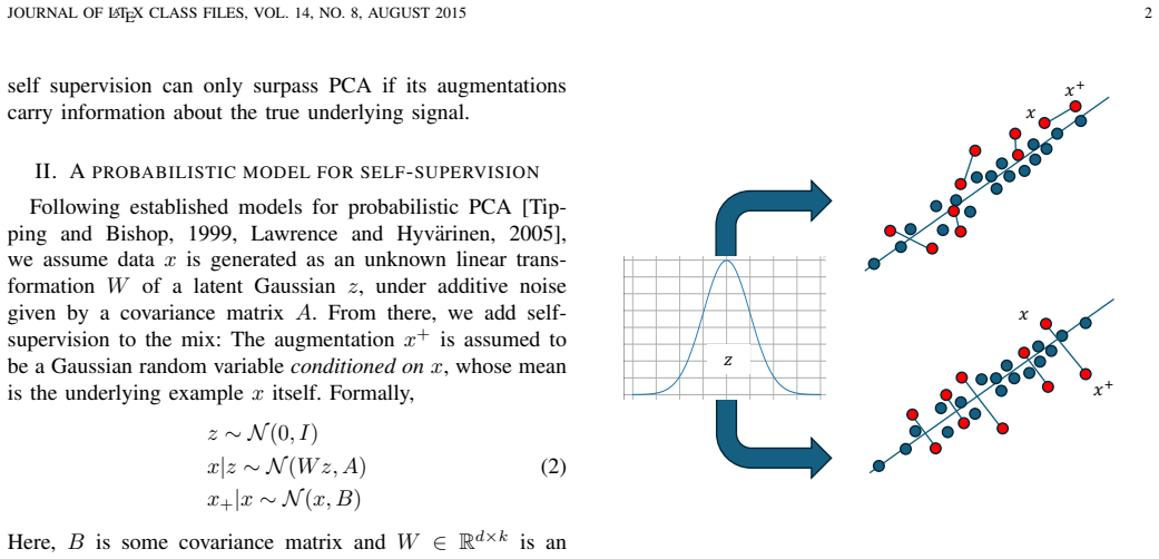
Under the generative model $z \sim N(0,I)$, $x|z \sim N(Wz,A)$, $x^+|x \sim N(x,B)$, with $W$ having orthonormal columns, the paper derives the exact log-likelihood of the observed positive pairs and analyzes its maximizer. Proposition 2 states that when $A=\sigma^2 I$ and $B=\epsilon^2 I$, the MLE of $W$ is the subspace spanned by the top $k$ eigenvectors of $S_x=\sum_i x_i x_i^\top$, so SSL collapses to PCA. Proposition 3 states that when $A=\rho I-WW^\top$ and $B=\gamma I-WW^\top$ with $\rho,\gamma>1$, the MLE is the top-$k$ eigenvector subspace of $-S_\Delta$, where $S_\Delta=\sum_i (x_i-x_i^+)(x_i-x_i^+)^\top$; this is the minimizer of the non-contrastive loss (1). The paper reads this as a probabilistic explanation of when self-supervision beats PCA: the augmentations must leave the signal direction $W$ unperturbed and add noise only in the orthogonal complement.

Load-bearing premise

The load-bearing premise is that augmentation noise has zero covariance along the signal subspace, $B=\gamma I-WW^\top$; if positive-pair differences have any variance in the $W$ direction, the exact equality between the MLE and the non-contrastive loss breaks down, and the authors concede this condition is too strong for real augmentations.

Editorial extensions

If this is right

If the orthogonal-noise model holds, the simple non-contrastive loss is not a heuristic regularizer but the score of a well-specified probabilistic model for the signal subspace.
The same model interpolates between PCA and SSL: the isotropic choice $B=\epsilon^2 I$ yields PCA, and the orthogonal choice $B=\gamma I-WW^\top$ yields the non-contrastive loss, so the augmentation distribution decides which classical estimator is being approximated.
The paper's remark that Gaussian input noise can still be a useful augmentation in deep models follows because a nonlinear feature map $\phi$ need not preserve Gaussianity of the noise in the function space where the linear embedding acts.
Because the likelihood is closed form, the model enables Bayesian inference over $W$, turning the SSL embedding into a posterior distribution that can propagate uncertainty to downstream predictors.

Reading between the lines

Editorial extensions of the paper, not claims the author makes directly.

The authors leave a relaxation implicit: replacing $B=\gamma I-WW^\top$ with $B=\gamma I-WW^\top+\alpha WW^\top$ should make the MLE interpolate between the non-contrastive loss and a PCA-like objective as $\alpha$ grows, quantifying how much semantic faithfulness SSL needs.
A practical diagnostic follows that the paper does not state: given a learned $W$ and a fixed augmentation pipeline, the projection of $\operatorname{Cov}(x-x^+)$ onto the signal subspace should predict how much SSL outperforms PCA, and can be measured on real datasets.
The same block-covariance derivation might extend to other SSL losses such as variance-invariance-covariance regularizers, but the paper only treats the squared-distance loss.

Share X Bluesky LinkedIn Reddit HN

Signed reviews

No signed human review yet.

Editorial analysis

A structured set of objections, weighed in public.

Desk editor's note, referee report, and a circularity audit.

Desk Editor's Note

read the letter

First, the main thing you should know: the stress-test note is right, and the paper is still a solid short theoretical result. The MLE-to-non-contrastive-loss equivalence in Prop. 3 is mathematically correct, but it depends on A = ρI − WW^T just as much as on B = γI − WW^T. The proof works because setting A this way makes the marginal covariance of x equal to ρI, so the data term Tr((WW^T + A)^−1 S_x) is constant in W. If A were isotropic σ²I, the MLE would solve a tradeoff between PCA variance and invariance, not reduce to loss (1). Section VI flags the orthogonal-noise assumption on B as strong, but it does not explicitly flag A, which is equally load-bearing and equally unrealistic. Section II's comment that 'whenever A perturbs the spectrum' hints at the issue but stops short of stating the implication. This is a scope limitation, not an internal inconsistency: the theorem is true as stated.

What is actually new: as far as I can tell, this is the first generative model that explicitly models positive-pair creation and whose MLE recovers the simple non-contrastive loss. Proposition 2 (isotropic noise → PCA) and Proposition 3 (orthogonal noise → non-contrastive loss) are clean, self-contained, and algebraically correct. The log-determinant constancy argument is valid, the Woodbury computations check out, and there is no circular fitting. The authors deserve credit for a proof-of-concept that answers a real question in the SSL theory literature.

Soft spots beyond the A-asymmetry: the abstract's word 'approaches' is vague, and the intro's PCA model formula has a typo (x|z should be Wz + μ, not Wx + μ). The simulations lack error bars, but they are only illustrative. None of these touches the central theorem.

Who this is for: readers interested in probabilistic justifications for linear non-contrastive SSL. The practical impact on deep SSL is indirect, and the authors are appropriately modest about that. I think the paper deserves a serious referee; it would fit a short-paper or workshop venue. I would recommend asking the authors to broaden the limitation discussion to include A and to soften 'natural' when describing the model.

Recommendation: accept for peer review, with minor revisions expected.

Referee Report

2 major / 6 minor

Summary. The paper proposes a latent-variable generative model for self-supervised learning, z~N(0,I), x|z~N(Wz,A), x+|x~N(x,B), with W having orthonormal columns. It derives the closed-form log-likelihood (Lemma 1) and shows that the MLE is PCA under isotropic noise covariances A=σ²I, B=ε²I (Proposition 2), and is the minimizer of the simple non-contrastive loss ||W^T x - W^T x+||² under covariances A=ρI-WW^T, B=γI-WW^T (Proposition 3). Simulations illustrate the two regimes, a Gaussian-mixture variant is experimented on, and a Bayesian extension is mentioned.

Significance. The strength of the paper is that Proposition 3 is a correct, explicit example of a maximum likelihood estimator that coincides with a non-contrastive SSL objective, which is a useful conceptual bridge and a clean theoretical observation. The algebraic derivations are sound and the model is simple enough to be checked by hand. The significance is tempered by the fact that the exact equivalence requires both noise covariances to be prescribed as functions of W, so the model is carefully tuned rather than a fully natural generative account of SSL; nevertheless, the paper makes a clear, falsifiable claim and the simulations are easy to reproduce.

major comments (2)

[Section VI, Proposition 3] The exact recovery of the non-contrastive loss in Proposition 3 requires not only B=γI-WW^T but also A=ρI-WW^T. In the proof, the lower block of Σ^{-1} becomes ρ^{-1}I only because WW^T+A=ρI, so the data term Tr((WW^T+A)^{-1}Sx) is independent of W. If A were the isotropic σ²I used in Proposition 2, the log-likelihood would contain a positive trace term from Sx and a negative trace term from SΔ, yielding an MLE that balances PCA variance against non-contrastive invariance rather than minimizing loss (1). Section VI flags the orthogonality assumption on B as strong, but it does not acknowledge that A is equally engineered and equally load-bearing. Please state this explicitly and either provide the general solution for A=σ²I, B=γI-WW^T or qualify the claim that the model is a natural statistical model for non-contrastive learning.
[Section II, example 2] The sentence 'Whenever A perturbs the spectrum of WW^T, the MLE is no longer given by the PCA solution' is not accurate as stated. With A=σ²I and B=γI-WW^T, the isotropic A also perturbs the spectrum of WW^T, and the resulting MLE is neither the PCA solution nor the minimizer of (1), but the hybrid described in the previous comment. This sentence should be replaced by a precise statement of how A and B jointly determine the objective, since the paper's 'interplay between noise and augmentations' narrative is only demonstrated at the two specially chosen covariance pairs.

minor comments (6)

[Introduction] The PCA generative formula reads 'x|z ∼ N(W x+ µ, σ²I)' but should be 'x|z ∼ N(Wz+µ, σ²I)'.
[Abstract, Proposition 3] The abstract says the MLE 'approaches' a simple non-contrastive loss; under the stated orthogonal covariance model it is exactly the minimizer, so 'is exactly' would be more accurate.
[Section II, example 2] The motivating example writes B=Id-WW^T, which is singular, whereas Proposition 3 requires γ>1; please clarify that this is a limiting or informal version of the orthogonal noise model.
[Section VI] The limitation statement says the positive pairs (x,x+) 'lie exactly along a subspace orthogonal to the signal direction,' but under the model it is the augmentation noise x+-x that has reduced (or in the limit zero) variance along W; the positive samples themselves retain the signal component of x. Please rephrase.
[Section IV, Figures 2 and 3] The simulations average over 1000 initializations but show no error bars or variance information; please include a measure of spread. Also describe how ẑ is estimated from W in the definitions of L_SSL and L_PCA.
[Throughout] There are small typos, e.g., 'Let us give ab brief recap' should be 'a brief recap,' and the caption of Figure 2 says 'isotropic nose model' instead of 'noise model.'

Circularity Check

0 steps flagged · score 0.0 of 10

No circularity: the MLE-to-SSL equivalence is derived from the stated generative model, not assumed.

full rationale

The paper's central claim is a mathematical equivalence: for the specific generative model (2) with A = ρI − WW^T and B = γI − WW^T, the MLE over orthonormal columns W is exactly the minimizer of the non-contrastive loss (Proposition 3). This result is derived from the likelihood in Lemma 1 and Proposition 3 using standard Gaussian identities and Woodbury's formula; nothing is fitted to data and then renamed as a prediction. The covariance choices are deliberately engineered to make the data term independent of W, leaving only the augmentation-difference term, but that is a modeling assumption rather than a circular step: the loss is not an input to the derivation, it is the output. The paper does not rely on any self-citation for the main equivalence; the only self-citation (Esser et al., 2023) appears in related work on dimension collapse and is not load-bearing. Section VI explicitly acknowledges the strength of the orthogonal-noise assumption, which is a realism concern, not a circularity. The derivation chain is self-contained and the result follows from the stated assumptions, so no circularity is present.

Assumptions & free parameters 4 free parameters · 6 assumptions · 0 invented entities

The derivation is self-contained given the Gaussian model. The special covariance structures A and B are the main assumptions; they are not estimated from data. No new physical or mathematical entities are introduced; the latent variable z is standard probabilistic PCA. The four scalar noise parameters are hand-chosen constants, but the central equivalence does not depend on their specific values.

free parameters (4)

sigma^2 (isotropic observation noise variance) = not fitted; any sigma^2 > 0
Appears in Proposition 2; the PCA result holds for all positive sigma^2.
epsilon^2 (isotropic augmentation noise variance) = not fitted; any epsilon^2 > 0
Appears in Proposition 2; cancels from the optimization because it is independent of W.
rho (orthogonal noise scale for observation covariance A) = not fitted; simulation uses 1.01, any rho > 1
Appears in Proposition 3; required for positive definiteness of A=rho I - W W^T, does not affect the resulting loss.
gamma (orthogonal noise scale for augmentation covariance B) = not fitted; simulation uses 1.01, any gamma > 1
Appears in Proposition 3; required for positive definiteness of B=gamma I - W W^T, does not affect the resulting loss.

assumptions (6)

domain assumption Data are generated by z ~ N(0,I), x|z ~ N(Wz,A), x+|x ~ N(x,B) (Eq. (2)).
This Gaussian structure is the entire statistical model; Lemma 1 computes the likelihood from it.
domain assumption W has orthonormal columns.
Stated after Eq. (1) and used in Propositions 2 and 3 to keep determinant terms constant and to define the embedding.
ad hoc to paper Noise covariances take the isotropic forms A=sigma^2 I, B=epsilon^2 I.
Proposition 2 uses these to show the MLE reduces to PCA.
ad hoc to paper Noise covariances take the orthogonal forms A=rho I - W W^T, B=gamma I - W W^T with rho, gamma > 1.
Proposition 3 uses these so the log-determinant is constant and the trace term becomes the non-contrastive loss.
domain assumption The n positive pairs are independent with independent latent variables z_i.
Lemma 1 factors the log-likelihood into a sum over i.
standard math Standard Gaussian integration, matrix determinant lemma, and Woodbury identity.
Used without proof in Lemma 1 and Propositions 2 and 3.

how reviews work

0 comments

Cite this review

Pith. "Pith review of A Probabilistic Model for Non-Contrastive Learning." pith.science (2026). https://pith.science/paper/3OC3MVNV

@misc{pith2026250113031,
  author       = {Pith},
  title        = {Pith review of: A Probabilistic Model for Non-Contrastive Learning},
  year         = {2026},
  howpublished = {\url{https://pith.science/paper/3OC3MVNV}},
  note         = {Machine review of arXiv:2501.13031}
}

read the original abstract

Self-supervised learning (SSL) aims to find meaningful representations from unlabeled data by encoding semantic similarities through data augmentations. Despite its current popularity, theoretical insights about SSL are still scarce. For example, it is not yet known whether commonly used SSL loss functions can be related to a statistical model, much in the same as OLS, generalized linear models or PCA naturally emerge as maximum likelihood estimates of an underlying generative process. In this short paper, we consider a latent variable statistical model for SSL that exhibits an interesting property: Depending on the informativeness of the data augmentations, the MLE of the model either reduces to PCA, or approaches a simple non-contrastive loss. We analyze the model and also empirically illustrate our findings.

Figures

Figures reproduced from arXiv: 2501.13031 by the authors.

**Figure 1.** Model Illustration. Data x is generated from a latent Gaussian, which is mapped linearly to a higher-dimensional space. Then, positive samples x + are generated as Gaussians conditioned on x. Depending on the covariance structure, we either recover an isotropic noise model (above) or the orthogonal noise model (below). In the latter, the positive pairs lie in a subspace orthogonal to the underlying signal direction.… view at source ↗

**Figure 2.** Numerical analysis of the theoretical setting. Plotted is [PITH_FULL_IMAGE:figures/full_fig_p004_2.png] view at source ↗

**Figure 3.** Orthogonal noise model with GMM latent space. [PITH_FULL_IMAGE:figures/full_fig_p004_3.png] view at source ↗

Discussion (0). Continue with ORCID to comment.

Reference graph

Works this paper leans on

23 extracted references · 18 canonical work pages

[1]

11em plus .33em minus .07em 4000 4000 100 4000 4000 500 `\.=1000 = #1 \@IEEEnotcompsoconly \@IEEEcompsoconly #1 * [1] 0pt [0pt][0pt] #1 * [1] 0pt [0pt][0pt] #1 * \| ** #1 \@IEEEauthorblockNstyle \@IEEEcompsocnotconfonly \@IEEEauthorblockAstyle \@IEEEcompsocnotconfonly \@IEEEcompsocconfonly \@IEEEauthordefaulttextstyle \@IEEEcompsocnotconfonly \@IEEEauthor...

work page
[2]

a ckinger, and Roopak Shah. Signature verification using a

Jane Bromley, Isabelle Guyon, Yann LeCun, Eduard S \"a ckinger, and Roopak Shah. Signature verification using a" siamese" time delay neural network. Advances in neural information processing systems, 1993

work page 1993
[3]

Self-supervised learning of pretext-invariant representations

Ishan Misra and Laurens van der Maaten. Self-supervised learning of pretext-invariant representations. In Proceedings of the IEEE/CVF Conference on Computer Vision and Pattern Recognition, 2020

work page 2020
[4]

Self-supervised video representation learning with odd-one-out networks

Basura Fernando, Hakan Bilen, Efstratios Gavves, and Stephen Gould. Self-supervised video representation learning with odd-one-out networks. In IEEE conference on computer vision and pattern recognition, 2017

work page 2017
[5]

A simple framework for contrastive learning of visual representations

Ting Chen, Simon Kornblith, Mohammad Norouzi, and Geoffrey Hinton. A simple framework for contrastive learning of visual representations. In International conference on machine learning. PMLR, 2020

work page 2020
[6]

wav2vec: Unsupervised pre-training for speech recognition, 2019

Steffen Steffen, Alexei Baevski, Ronan Collobert, and Michael Auli. wav2vec: Unsupervised pre-training for speech recognition, 2019

work page 2019
[7]

Representation learning: A review and new perspectives

Yoshua Bengio, Aaron Courville, and Pascal Vincent. Representation learning: A review and new perspectives. IEEE transactions on pattern analysis and machine intelligence, 2013

work page 2013
[8]

Christopher M. Bishop. Pattern Recognition and Machine Learning (Information Science and Statistics). Springer-Verlag, 2006

2006

Show all 23 references

[9]

Probabilistic principal component analysis

Michael E Tipping and Christopher M Bishop. Probabilistic principal component analysis. Journal of the Royal Statistical Society Series B: Statistical Methodology, 61 0 (3): 0 611--622, 1999

1999
[10]

Probabilistic non-linear principal component analysis with gaussian process latent variable models

Neil Lawrence and Aapo Hyv \"a rinen. Probabilistic non-linear principal component analysis with gaussian process latent variable models. Journal of machine learning research, 6 0 (11), 2005

2005
[11]

Barlow twins: Self-supervised learning via redundancy reduction

Jure Zbontar, Li Jing, Ishan Misra, Yann LeCun, and St \'e phane Deny. Barlow twins: Self-supervised learning via redundancy reduction. In International conference on machine learning. PMLR, 2021

2021
[12]

Vicreg: Variance-invariance-covariance regularization for self-supervised learning

Adrien Bardes, Jean Ponce, and Yann LeCun. Vicreg: Variance-invariance-covariance regularization for self-supervised learning. arXiv preprint arXiv:2105.04906, 2021

2021 arXiv
[13]

Toward understanding the feature learning process of self-supervised contrastive learning

Zixin Wen and Yuanzhi Li. Toward understanding the feature learning process of self-supervised contrastive learning. In International Conference on Machine Learning. PMLR, 2021

2021
[14]

Towards a unified theoretical understanding of non-contrastive learning via rank differential mechanism

Zhijian Zhuo, Yifei Wang, Jinwen Ma, and Yisen Wang. Towards a unified theoretical understanding of non-contrastive learning via rank differential mechanism. In The Eleventh International Conference on Learning Representations, 2023

2023
[15]

Contrasting the landscape of contrastive and non-contrastive learning

Ashwini Pokle, Jinjin Tian, Yuchen Li, and Andrej Risteski. Contrasting the landscape of contrastive and non-contrastive learning. arXiv preprint arXiv:2203.15702, 2022

2022 arXiv
[16]

Representation learning dynamics of self-supervised models

Pascal Esser, Satyaki Mukherjee, and Debarghya Ghoshdastidar. Representation learning dynamics of self-supervised models. Transactions on Machine Learning Research, 2023

2023
[17]

A theoretical analysis of contrastive unsupervised representation learning

Sanjeev Arora, Hrishikesh Khandeparkar, Mikhail Khodak, Orestis Plevrakis, and Nikunj Saunshi. A theoretical analysis of contrastive unsupervised representation learning. In International Conference on Machine Learning, 2019

2019
[18]

Why do pretrained language models help in downstream tasks? an analysis of head and prompt tuning

Colin Wei, Sang Michael Xie, and Tengyu Ma. Why do pretrained language models help in downstream tasks? an analysis of head and prompt tuning. In Advances in Neural Information Processing Systems, 2021

2021
[19]

Bayesian self-supervised contrastive learning

Bin Liu and Bang Wang. Bayesian self-supervised contrastive learning. arXiv preprint arXiv:2301.11673, 2023

2023 arXiv
[20]

Probabilistic self-supervised learning via scoring rules minimization

Amirhossein Vahidi, Simon Scho er, Lisa Wimmer, Yawei Li, Bernd Bischl, Eyke H \"u llermeier, and Mina Rezaei. Probabilistic self-supervised learning via scoring rules minimization. arXiv preprint arXiv:2309.02048, 2023

2023 arXiv
[21]

A probabilistic model to explain self-supervised representation learning

Alice Bizeul, Bernhard Sch \"o lkopf, and Carl Allen. A probabilistic model to explain self-supervised representation learning. arXiv preprint arXiv:2402.01399, 2024

2024 arXiv
[22]

Contrastive learning inverts the data generating process

Roland S Zimmermann, Yash Sharma, Steffen Schneider, Matthias Bethge, and Wieland Brendel. Contrastive learning inverts the data generating process. In International Conference on Machine Learning. PMLR, 2021

2021
[23]

Representation learning with contrastive predictive coding

Aaron van den Oord, Yazhe Li, and Oriol Vinyals. Representation learning with contrastive predictive coding. In Proceedings of the 32nd International Conference on Neural Information Processing Systems, 2018

2018

Pith tools

Reviewed August 10, 2026 · model on record in the stance chip above.

[1] [1]

11em plus .33em minus .07em 4000 4000 100 4000 4000 500 `\.=1000 = #1 \@IEEEnotcompsoconly \@IEEEcompsoconly #1 * [1] 0pt [0pt][0pt] #1 * [1] 0pt [0pt][0pt] #1 * \| ** #1 \@IEEEauthorblockNstyle \@IEEEcompsocnotconfonly \@IEEEauthorblockAstyle \@IEEEcompsocnotconfonly \@IEEEcompsocconfonly \@IEEEauthordefaulttextstyle \@IEEEcompsocnotconfonly \@IEEEauthor...

work page

[2] [2]

a ckinger, and Roopak Shah. Signature verification using a

Jane Bromley, Isabelle Guyon, Yann LeCun, Eduard S \"a ckinger, and Roopak Shah. Signature verification using a" siamese" time delay neural network. Advances in neural information processing systems, 1993

work page 1993

[3] [3]

Self-supervised learning of pretext-invariant representations

Ishan Misra and Laurens van der Maaten. Self-supervised learning of pretext-invariant representations. In Proceedings of the IEEE/CVF Conference on Computer Vision and Pattern Recognition, 2020

work page 2020

[4] [4]

Self-supervised video representation learning with odd-one-out networks

Basura Fernando, Hakan Bilen, Efstratios Gavves, and Stephen Gould. Self-supervised video representation learning with odd-one-out networks. In IEEE conference on computer vision and pattern recognition, 2017

work page 2017

[5] [5]

A simple framework for contrastive learning of visual representations

Ting Chen, Simon Kornblith, Mohammad Norouzi, and Geoffrey Hinton. A simple framework for contrastive learning of visual representations. In International conference on machine learning. PMLR, 2020

work page 2020

[6] [6]

wav2vec: Unsupervised pre-training for speech recognition, 2019

Steffen Steffen, Alexei Baevski, Ronan Collobert, and Michael Auli. wav2vec: Unsupervised pre-training for speech recognition, 2019

work page 2019

[7] [7]

Representation learning: A review and new perspectives

Yoshua Bengio, Aaron Courville, and Pascal Vincent. Representation learning: A review and new perspectives. IEEE transactions on pattern analysis and machine intelligence, 2013

work page 2013

[8] [8]

Christopher M. Bishop. Pattern Recognition and Machine Learning (Information Science and Statistics). Springer-Verlag, 2006

2006