REVIEW 3 major objections 5 minor 88 references
Handling Missing Data in Downstream Tasks With Distribution-Preserving Guarantees
T0 review · 3 major / 5 minor · reviewed 2026-08-10 · deepseek-v4-flash
Pith's one-line read F3I is a fast K-nearest-neighbor imputer that provably preserves the data distribution while bounding imputation error.
desk verdict A genuinely new and fast KNN-based imputer with careful bounds, but the 'distribution-preserving guarantees' in the title are not what the theorems prove. read the letter →
The pith
A machine-rendered reading of the paper's core claim, the machinery that carries it, and where it could break.
The reading
What carries the argument
The central object is the function $G(\alpha, X) = \frac{1}{N}\sum_{i\le N}\log\frac{D_0(x_i(\alpha))}{D_0(x_i)} - \eta\|\alpha\|_2^2$, where $\alpha$ is a simplex of $K$ weights, $x_i(\alpha)$ is the convex combination of the $K$ nearest neighbors of sample $i$, and $D_0$ is a Gaussian kernel density estimate over the initially imputed points. The function quantifies how much more probable the reweighted imputation is than the current guess. Concavity of $G$ for small regularization $\eta$ and large enough bandwidth $h$ turns weight learning into convex optimization; Lipschitz gradients let the authors apply AdaHedge's no-regret bound and, with PCGrad, a joint-training bound. The telescoping sum identity is what connects per-round optimization to an end-to-end log-density improvement.
What would settle it
Take any dataset generated exactly by the paper's Algorithm 3 with the stated Gaussian assumptions and run F3I for all three missingness mechanisms across many seeds; if the imputation MSE ever exceeds the claimed bound $O((\sigma_{\mathrm{miss}})^2 + \ln N / F)$ or the cumulative regret exceeds $C_{\mathrm{AH}}\sqrt{t} + H_{\mathrm{miss}} h^{-1} t$ at the stated $1-1/N$ confidence, the theorem fails. A more behavior-level test, valid even where the assumptions fail, is to generate strongly correlated features and compare the probability of F3I's imputed values under the true data density with the probability of the initial KNN guesses: if maximizing $G$ lowers true-density probability, the algorithm is not preserving the distribution it claims to preserve.
Extended reading notes
Core claim
On its own terms, the discovery is that the neighbor weights in a K-nearest-neighbor imputer can be tuned online so that imputed values are, with high probability, at least as probable under the data density as the initial guesses, while the mean squared error stays controlled. F3I formalizes distribution preservation through the ratio $D_0(x_i(\alpha))/D_0(x_i)$ inside a Gaussian kernel density estimate, and the paper proves this objective is concave with a Lipschitz gradient. The no-regret learner AdaHedge then supplies the weight sequence, and the paper's Theorem 4.4 bounds the cumulative regret of that sequence against the a posteriori best fixed weights; Theorem 4.2 bounds the MSE. The proofs use a high-probability concentration bound on the initial KNN error, which is where the independence-in-Gaussians assumption enters.
Load-bearing premise
The load-bearing premise is that every entry of the complete data matrix is drawn independently from a Gaussian with the same spread, meaning the observed features carry no information about a missing value; if real data have correlated features or heavy tails, the paper's mathematical guarantees stop applying.
Editorial extensions
If this is right
- Under the assumed Gaussian model, the imputation MSE is $O((\sigma_{\mathrm{miss}})^2 + \ln N / F)$ with probability $1-1/N$, so larger data variance worsens imputation while more features or more samples improve it.
- The cumulative regret against the best fixed neighbor weights is $C_{\mathrm{AH}}\sqrt{t} + H_{\mathrm{miss}} h^{-1} t$, meaning the online learner is not asymptotically worse than the optimal static weight vector, apart from a linear term that the paper attributes to using a fixed initial density estimate.
- The joint-training version PCGrad-F3I has the same guarantee with a classifier loss: setting $\beta=0$ recovers the imputation-only bound and $\beta=1$ recovers the classical AdaHedge regret bound on the downstream loss.
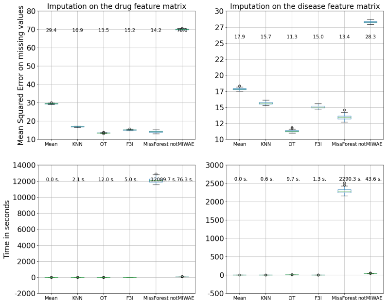
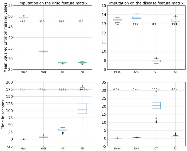
- Because weight updates are single online steps, the per-iteration cost is $O(NK(\log N + F))$ after an $O(FN\log N)$ preprocessing step, which is why the method runs orders of magnitude faster than graph, diffusion, and GAN imputers in the experiments.
Reading between the lines
- If the independence assumption B.1 is violated, as it is in most real data, the theoretical bounds do not apply, and the density-ratio objective may actually favor shrinking values toward the mean, which would reduce variance rather than preserve the data distribution; the real-data experiments, not the theorems, carry the practical case.
- Re-estimating the kernel density on the currently imputed points at each round, which the paper names as future work, would likely replace the linear $H_{\mathrm{miss}} h^{-1} t$ regret term with a vanishing term and make the distribution-preservation guarantee match the objective being optimized.
- The same online-reweighting scheme could be combined with any base imputer whose output is a convex combination with Lipschitz-continuous gradient, potentially extending the guarantees to linear or shallow-network imputers without changing the regret analysis.
Editorial analysis
A structured set of objections, weighed in public.
Referee Report
Summary. The manuscript introduces F3I, an iterative K-nearest-neighbor imputation method that learns neighbor weights via AdaHedge to maximize a concave kernel-density log-ratio objective G. It also introduces PCGrad-F3I for joint imputation and classification. The paper states high-probability bounds on imputation MSE (Theorem 4.2), on cumulative regret against the best fixed weights for the 'true' objective G* (Theorem 4.4), and a joint-training regret bound (Theorem 5.1). Experiments on real and synthetic data, including drug repurposing and MNIST, are used to support claims of competitive accuracy and much lower runtime than deep-learning baselines.
Significance. F3I is a simple, fast, and reproducible imputer; the theoretical machinery (AdaHedge regret, concentration bounds on sub-Gaussian imputation errors) is internally coherent under Assumptions B.1-B.6, and the experimental study is extensive. The main advertised value is a distribution-preserving imputer with guarantees. However, the advertised distribution-preservation property is not what is proved: Theorem 4.4 bounds regret of a pointwise log-density ratio, which is a mode-seeking objective, and under the paper's independent-Gaussian assumption this objective shrinks imputed values toward feature means rather than preserving the true distribution. The MSE bound in Theorem 4.2 does not depend on the learned weights and therefore does not establish a benefit of F3I over initial KNN imputation. These issues substantially weaken the paper's central claim.
major comments (3)
- [Section 3.2 and Theorem 4.4] The title and abstract promise 'distribution-preserving guarantees,' but the quantity bounded in Theorem 4.4 is the cumulative regret of G*(alpha,X)=1/N sum_i log(D*(x_i(alpha))/D*(x_i))-eta||alpha||^2. This is a pointwise log-density ratio, not a divergence between the imputed and true distributions. Maximizing G is mode-seeking: it moves imputed points toward high-density regions of D* rather than sampling from D*. Under Assumption B.1 the features are independent Gaussians, so observed coordinates are independent of a missing coordinate; the MSE-optimal imputation is the feature mean, and every non-degenerate convex combination of K neighbors has excess variance. The density objective then favors weights that shrink imputed values toward the mean. This is the opposite of preserving the data distribution, and it explains why mean imputation is reported as competitive or better on MCAR/MAR synthetic data (Appendix H.1.2). A low regret bound with respect to G* therefore does not substantiate the paper's central distribution-preservation claim.
- [Theorem 4.2 and Appendix D] The MSE bound is essentially a bound on the initial KNN imputation, not on the learned imputation weights. In the proof of Theorem D.1, Jensen's inequality is applied to an arbitrary alpha in Delta_K, and the resulting bound depends only on max_{i,j}||(x0)_j-(x*)_i||^2 via Corollary G.6; none of the steps use the F3I updates or the objective G. Consequently, the theorem does not show that F3I improves over uniform-KNN initial guesses, and it is not a distribution-preservation result. If the intended statement is 'any convex combination of the K initial neighbors has MSE O((sigma_miss)^2+ln N/F),' the theorem should say so explicitly.
- [Section 5, Eq. (2), and Assumption B.8] Theorem 5.1 is conditional on Assumption B.8, which essentially assumes the full set of hypotheses of Theorem 2 of Yu et al. (PCGrad), including the angle condition, a step-size condition, and the Hessian inequality H(-G,alpha,alpha') >= w||g||^2. The appendix verifies convexity and Lipschitz continuity of -G (Proposition C.5 and Lemma F.1), but it does not verify the additional angle and curvature conditions for the specific F3I objective and logistic loss. As stated, the theorem is an application of an external result under unverified hypotheses. The authors should either prove those hypotheses for their setting or mark them explicitly as assumptions on the loss and step-size, rather than presenting Theorem 5.1 as a derived guarantee of PCGrad-F3I.
minor comments (5)
- [Proposition C.2] Proposition C.2 states that eta<4KN suffices for strict concavity, but the proof around Eq. (4) uses eta<4S^2K=4K; the statement and proof need to be reconciled.
- [Algorithm 2] Algorithm 2's neighbor-selection line ('1,2,...,K arg min_{j<=N} ...') is difficult to parse; it should explicitly say that K indices are chosen by increasing Chebyshev distance to x.
- [Assumption B.1] Assumption B.1's text writes (x*)_i ~ N_F(mu_f, sigma^2 I) with a scalar mu_f, while Algorithm 3 samples each coordinate from N(mu_f, sigma^2); use a vector mu in R^F consistently.
- [Figure 1 caption] Figure 1 caption contains a typo: 'Emprical' should be 'Empirical.'
- [Table 16 caption] The statement in Table 16's caption that TDM failed on Gottlieb is irrelevant because TDM is not among the selected baselines in that table; remove or clarify.
Circularity Check
No significant circularity: the theoretical guarantees are derived from stated distributional assumptions and external regret/concentration theorems, not from fitting or self-citation.
full rationale
The paper's central claims (Theorems 4.2, 4.4, and 5.1) are proved from the explicit Assumptions B.1-B.6 using external results: AdaHedge's regret bound [24], Bernstein/subgaussian concentration (Technical lemmas 1-3, Corollary G.6, from Vershynin [68]), and PCGrad's convergence theorem [35]. The constants Cmiss, Hmiss, and CAH are derived analytically from these ingredients, not fitted to the target MSE or regret values. The distribution-preservation objective G is indeed defined by the authors, but the regret bound in Theorem 4.4 is stated and proved for G*, which uses the true, unavailable density D* rather than the estimated D0, and the proof explicitly bounds the gap between G and G* in high probability; thus the result is not the training objective by construction. The only self-references are dataset citations ([48], [69]) used as experimental inputs, which are not load-bearing for the theory. The paper's own limitation statement (Section 7) acknowledges that the theoretical assumptions are strong; this is a correctness caveat, not a circular step. The mode-seeking interpretation of the log-density objective is a conceptual concern about whether the quantity being bounded matches the title's promise, but it does not make the derivation circular.
Assumptions & free parameters
free parameters (4)
- bandwidth h =
smallest positive root of the cubic in Eq. (4)
- regularization eta =
0.001 in Table 3, tuned to 0.053 on MNIST
- number of neighbors K =
5 on synthetic data, 17 on MNIST, 12 on PREDICT
- downstream weight beta =
0.71 on MNIST, 0.246 on PREDICT, 0.5 in synthetic validation
assumptions (6)
- domain assumption Assumption B.1: every complete-data entry is an independent Gaussian draw with feature-specific mean and common variance sigma^2.
- domain assumption Assumptions B.2-B.4: missing indicators follow MCAR, a logistic-style MAR, or Gaussian self-masking MNAR.
- domain assumption Assumption B.5: at least K samples are observed for every feature.
- domain assumption Assumption B.6: all feature vectors have bounded norm and are renormalized so S = 1.
- ad hoc to paper Assumption B.8: the PCGrad conditions from Theorem 2 of Yu et al. hold, including a step-size and angle condition.
- standard math Standard concentration and regret results: Bernstein's inequality, subgaussian concentration, and AdaHedge regret bounds.
Cite this review
Pith. "Pith review of Handling Missing Data in Downstream Tasks With Distribution-Preserving Guarantees." pith.science (2026). https://pith.science/paper/O556WQOW
@misc{pith2026250113786,
  author       = {Pith},
  title        = {Pith review of: Handling Missing Data in Downstream Tasks With Distribution-Preserving Guarantees},
  year         = {2026},
  howpublished = {\url{https://pith.science/paper/O556WQOW}},
  note         = {Machine review of arXiv:2501.13786}
}
read the original abstract
Missing feature values are a significant hurdle for downstream machine-learning tasks such as classification. However, imputation methods for classification might be time-consuming for high-dimensional data, and offer few theoretical guarantees on the preservation of the data distribution and imputation quality, especially for not-missing-at-random mechanisms. First, we propose an imputation approach named F3I based on the iterative improvement of a K-nearest neighbor imputation, where neighbor-specific weights are learned through the optimization of a novel concave, differentiable objective function related to the preservation of the data distribution on non-missing values. F3I can then be chained to and jointly trained with any classifier architecture. Second, we provide a theoretical analysis of imputation quality and data distribution preservation by F3I for several types of missing mechanisms. Finally, we demonstrate the superior performance of F3I on several imputation and classification tasks, with applications to drug repurposing and handwritten-digit recognition data.
Figures


Figures from the paper (21 more)





Reference graph
Works this paper leans on
-
[1]
Inference and missing data
Donald B Rubin. Inference and missing data. Biometrika, 63(3):581–592, 1976
1976
-
[2]
Imputation for prediction: beware of diminishing returns
Marine Le Morvan and Gaël Varoquaux. Imputation for prediction: beware of diminishing returns. arXiv preprint arXiv:2407.19804, 2024
arXiv 2024
-
[3]
mice: Multivariate imputation by chained equations in r
Stef van Buuren and Karin Groothuis-Oudshoorn. mice: Multivariate imputation by chained equations in r. Journal of Statistical Software, 45(3):1–67, 2011. doi: 10.18637/jss.v045.i03
-
[4]
Missforest—non-parametric missing value imputation for mixed-type data
Daniel J Stekhoven and Peter Bühlmann. Missforest—non-parametric missing value imputation for mixed-type data. Bioinformatics, 28(1):112–118, 2012
2012
-
[5]
Geometry-and accuracy-preserving random forest proximities
Jake S Rhodes, Adele Cutler, and Kevin R Moon. Geometry-and accuracy-preserving random forest proximities. IEEE Transactions on Pattern Analysis and Machine Intelligence, 45(9): 10947–10959, 2023
2023
-
[6]
An intelligent missing data imputation tech- niques: A review
Kimseth Seu, Mi-Sun Kang, and HwaMin Lee. An intelligent missing data imputation tech- niques: A review. JOIV: International Journal on Informatics Visualization, 6(1-2):278–283, 2022
2022
-
[7]
Missing data imputation using optimal transport
Boris Muzellec, Julie Josse, Claire Boyer, and Marco Cuturi. Missing data imputation using optimal transport. In International Conference on Machine Learning, pages 7130–7140. PMLR, 2020
2020
-
[8]
Spectral regularization algorithms for learning large incomplete matrices
Rahul Mazumder, Trevor Hastie, and Robert Tibshirani. Spectral regularization algorithms for learning large incomplete matrices. The Journal of Machine Learning Research, 11:2287–2322, 2010
2010
Show all 88 references
-
[9]
Imputation of missing values in multi-view data
Wouter van Loon, Marjolein Fokkema, Frank de V os, Marisa Koini, Reinhold Schmidt, and Mark de Rooij. Imputation of missing values in multi-view data. Information Fusion, page 102524, 2024
2024
-
[10]
MIW AE: Deep generative modelling and imputation of incomplete data sets
Pierre-Alexandre Mattei and Jes Frellsen. MIW AE: Deep generative modelling and imputation of incomplete data sets. In Kamalika Chaudhuri and Ruslan Salakhutdinov, editors,Proceedings of the 36th International Conference on Machine Learning , volume 97 of Proceedings of Machin...
2019
-
[11]
not-{miwae}: Deep genera- tive modelling with missing not at random data
Niels Bruun Ipsen, Pierre-Alexandre Mattei, and Jes Frellsen. not-{miwae}: Deep genera- tive modelling with missing not at random data. In International Conference on Learning Representations, 2021. URL https://openreview.net/forum?id=tu29GQT0JFy. 10
2021
-
[12]
Miracle: Causally-aware imputation via learning missing data mechanisms
Trent Kyono, Yao Zhang, Alexis Bellot, and Mihaela van der Schaar. Miracle: Causally-aware imputation via learning missing data mechanisms. Advances in Neural Information Processing Systems, 34:23806–23817, 2021
2021
-
[13]
Hyperimpute: Generalized iterative imputation with automatic model selection
Daniel Jarrett, Bogdan C Cebere, Tennison Liu, Alicia Curth, and Mihaela van der Schaar. Hyperimpute: Generalized iterative imputation with automatic model selection. In International Conference on Machine Learning, pages 9916–9937. PMLR, 2022
2022
-
[14]
Pro- cessing of missing data by neural networks
Marek ´Smieja, Łukasz Struski, Jacek Tabor, Bartosz Zieli´nski, and Przemysław Spurek. Pro- cessing of missing data by neural networks. Advances in neural information processing systems, 31, 2018
2018
-
[15]
Analysis of multivariate missing data with nonignorable nonresponse
Gong Tang, Roderick JA Little, and Trivellore E Raghunathan. Analysis of multivariate missing data with nonignorable nonresponse. Biometrika, 90(4):747–764, 2003
2003
-
[16]
Estimation with incomplete data: The linear case
Karthika Mohan, Felix Thoemmes, and Judea Pearl. Estimation with incomplete data: The linear case. In Proceedings of the International Joint Conferences on Artificial Intelligence Organization, 2018
2018
-
[17]
Estimation and imputation in probabilistic principal component analysis with missing not at random data
Aude Sportisse, Claire Boyer, and Julie Josse. Estimation and imputation in probabilistic principal component analysis with missing not at random data. Advances in Neural Information Processing Systems, 33:7067–7077, 2020
2020
-
[18]
Neumiss networks: differentiable programming for supervised learning with missing values
Marine Le Morvan, Julie Josse, Thomas Moreau, Erwan Scornet, and Gaël Varoquaux. Neumiss networks: differentiable programming for supervised learning with missing values. Advances in Neural Information Processing Systems, 33:5980–5990, 2020
2020
-
[19]
Missing value estimation methods for dna microarrays
Olga Troyanskaya, Michael Cantor, Gavin Sherlock, Pat Brown, Trevor Hastie, Robert Tibshi- rani, David Botstein, and Russ B Altman. Missing value estimation methods for dna microarrays. Bioinformatics, 17(6):520–525, 2001
2001
-
[20]
A survey on missing data in machine learning
Tlamelo Emmanuel, Thabiso Maupong, Dimane Mpoeleng, Thabo Semong, Banyatsang Mphago, and Oteng Tabona. A survey on missing data in machine learning. Journal of Big data, 8:1–37, 2021
2021
-
[21]
On the performance of imputation techniques for missing values on healthcare datasets
Luke Oluwaseye Joel, Wesley Doorsamy, and Babu Sena Paul. On the performance of imputation techniques for missing values on healthcare datasets. arXiv preprint arXiv:2403.14687, 2024
2024 arXiv
-
[22]
Nearest neighbor imputation algorithms: a critical evaluation
Lorenzo Beretta and Alessandro Santaniello. Nearest neighbor imputation algorithms: a critical evaluation. BMC medical informatics and decision making, 16:197–208, 2016
2016
-
[23]
Prediction, learning, and games
Nicolo Cesa-Bianchi and Gábor Lugosi. Prediction, learning, and games. Cambridge university press, 2006
2006
-
[24]
Follow the leader if you can, hedge if you must
Steven De Rooij, Tim Van Erven, Peter D Grünwald, and Wouter M Koolen. Follow the leader if you can, hedge if you must. The Journal of Machine Learning Research, 15(1):1281–1316, 2014
2014
-
[25]
Bandit algorithms
Tor Lattimore and Csaba Szepesvári. Bandit algorithms. Cambridge University Press, 2020
2020
-
[26]
Richard Witmer, and Øystein Ore
Girolamo Cardano, T. Richard Witmer, and Øystein Ore. Ars magna, or, The rules of algebra. Dover, New York, 1968. ISBN 9780486678115; 0486678113
1968
-
[27]
Advances in collaborative filtering
Yehuda Koren, Steffen Rendle, and Robert Bell. Advances in collaborative filtering. Recom- mender systems handbook, pages 91–142, 2021
2021
-
[28]
Multidimensional binary search trees used for associative searching
Jon Louis Bentley. Multidimensional binary search trees used for associative searching. Com- mun. ACM, 18(9):509–517, sep 1975. ISSN 0001-0782. doi: 10.1145/361002.361007. URL https://doi.org/10.1145/361002.361007
1975
-
[29]
Gamification of pure exploration for linear bandits
Rémy Degenne, Pierre Ménard, Xuedong Shang, and Michal Valko. Gamification of pure exploration for linear bandits. In International Conference on Machine Learning, pages 2432–
-
[30]
Schapire
Peter Auer, Nicolò Cesa-Bianchi, Yoav Freund, and Robert E. Schapire. The nonstochastic multiarmed bandit problem. SIAM Journal on Computing, 32(1):48–77, 2002. doi: 10.1137/ S0097539701398375. URL https://doi.org/10.1137/S0097539701398375
2002 doi
-
[31]
What’sa good imputation to predict with missing values? Advances in Neural Information Processing Systems , 34: 11530–11540, 2021
Marine Le Morvan, Julie Josse, Erwan Scornet, and Gaël Varoquaux. What’sa good imputation to predict with missing values? Advances in Neural Information Processing Systems , 34: 11530–11540, 2021
2021
-
[32]
Optimal transport for structure learning under missing data
Vy V o, He Zhao, Trung Le, Edwin V Bonilla, and Dinh Phung. Optimal transport for structure learning under missing data. arXiv preprint arXiv:2402.15255, 2024
2024 arXiv
-
[33]
Naive imputation im- plicitly regularizes high-dimensional linear models
Alexis Ayme, Claire Boyer, Aymeric Dieuleveut, and Erwan Scornet. Naive imputation im- plicitly regularizes high-dimensional linear models. In International Conference on Machine Learning, pages 1320–1340. PMLR, 2023
2023
-
[34]
GradNorm: Gra- dient normalization for adaptive loss balancing in deep multitask networks
Zhao Chen, Vijay Badrinarayanan, Chen-Yu Lee, and Andrew Rabinovich. GradNorm: Gra- dient normalization for adaptive loss balancing in deep multitask networks. In Jennifer Dy and Andreas Krause, editors, Proceedings of the 35th International Conference on Machine Learning, vol...
2018
-
[35]
Gradient surgery for multi-task learning
Tianhe Yu, Saurabh Kumar, Abhishek Gupta, Sergey Levine, Karol Hausman, and Chelsea Finn. Gradient surgery for multi-task learning. In H. Larochelle, M. Ranzato, R. Hadsell, M.F. Balcan, and H. Lin, editors, Advances in Neural Information Processing Systems, volume 33, pages 5...
2020
-
[36]
Conflict-averse gradient descent for multi-task learning
Bo Liu, Xingchao Liu, Xiaojie Jin, Peter Stone, and Qiang Liu. Conflict-averse gradient descent for multi-task learning. Advances in Neural Information Processing Systems, 34:18878–18890, 2021
2021
-
[37]
William Wolberg, Olvi Mangasarian, Nick Street, and W. Street. Breast Cancer Wisconsin (Di- agnostic). UCI Machine Learning Repository, 1993. DOI: https://doi.org/10.24432/C5DW2B
1993 doi
-
[38]
Pedregosa, G
F. Pedregosa, G. Varoquaux, A. Gramfort, V . Michel, B. Thirion, O. Grisel, M. Blondel, P. Prettenhofer, R. Weiss, V . Dubourg, J. Vanderplas, A. Passos, D. Cournapeau, M. Brucher, M. Perrot, and E. Duchesnay. Scikit-learn: Machine learning in Python. Journal of Machine Learni...
2011
-
[39]
Heart Disease
Andras Janosi, William Steinbrunn, Matthias Pfisterer, and Robert Detrano. Heart Disease. UCI Machine Learning Repository, 1989. DOI: https://doi.org/10.24432/C52P4X
1989 doi
-
[40]
Datasets
selva86. Datasets. https://github.com/selva86/datasets/blob/master/ Ionosphere.csv, 2024
2024
-
[41]
Drug repositioning based on comprehensive similarity measures and bi-random walk algorithm
Huimin Luo, Jianxin Wang, Min Li, Junwei Luo, Xiaoqing Peng, Fang-Xiang Wu, and Yi Pan. Drug repositioning based on comprehensive similarity measures and bi-random walk algorithm. Bioinformatics, 32(17):2664–2671, 2016
2016
-
[42]
Gain: Missing data imputation using generative adversarial nets
Jinsung Yoon, James Jordon, and Mihaela Schaar. Gain: Missing data imputation using generative adversarial nets. In International conference on machine learning, pages 5689–5698. PMLR, 2018
2018
-
[43]
Handling Missing Data with Graph Representation Learning
Jiaxuan You, Xiaobai Ma, Yi Ding, Mykel J Kochenderfer, and Jure Leskovec. Handling Missing Data with Graph Representation Learning. In H. Larochelle, M. Ranzato, R. Hadsell, M. F. Bal- can, and H. Lin, editors, Advances in Neural Information Processing Systems, volume 33, pag...
2020
-
[44]
Rethinking the diffusion models for missing data imputation: A gradient flow perspective
Zhichao Chen, Haoxuan Li, Fangyikang Wang, Odin Zhang, Hu Xu, Xiaoyu Jiang, Zhihuan Song, and Hao Wang. Rethinking the diffusion models for missing data imputation: A gradient flow perspective. In The Thirty-eighth Annual Conference on Neural Information Processing Systems, 20...
2024
-
[45]
Remasker: Imputing tabular data with masked autoencoding
Tianyu Du, Luca Melis, and Ting Wang. Remasker: Imputing tabular data with masked autoencoding. arXiv preprint arXiv:2309.13793, 2023
2023 arXiv
-
[46]
Transformed distribution matching for missing value imputation
He Zhao, Ke Sun, Amir Dezfouli, and Edwin V Bonilla. Transformed distribution matching for missing value imputation. In International Conference on Machine Learning, pages 42159– 42186. PMLR, 2023
2023
-
[47]
LeCun, C
Y . LeCun, C. Cortes, and C.J.C. Burges. The mnist database of handwritten digits. https: //drive.google.com/file/d/1eEKzfmEu6WKdRlohBQiqi3PhW_uIVJVP/view, 1998
1998
-
[48]
Predict drug repurposing dataset
Clémence Réda. Predict drug repurposing dataset. doi: 10.5281/zenodo.7983090, 2023. URL https://doi.org/10.5281/zenodo.7983090
2023 doi
-
[49]
Billion-scale similarity search with gpus
Jeff Johnson, Matthijs Douze, and Hervé Jégou. Billion-scale similarity search with gpus. IEEE Transactions on Big Data, 7(3):535–547, 2019
2019
-
[50]
Locality preserving hashing
Kang Zhao, Hongtao Lu, and Jincheng Mei. Locality preserving hashing. In Proceedings of the AAAI conference on artificial intelligence, volume 28, 2014
2014
-
[51]
Locality preserving hashing
Yi-Hsuan Tsai and Ming-Hsuan Yang. Locality preserving hashing. In 2014 IEEE International Conference on Image Processing (ICIP), pages 2988–2992. IEEE, 2014
2014
-
[52]
Annoy: Approximate Nearest Neighbors in C++/Python , 2018
Erik Bernhardsson. Annoy: Approximate Nearest Neighbors in C++/Python , 2018. URL https://pypi.org/project/annoy/. Python package version 1.13.0
2018
-
[53]
Bore: Bayesian optimization by density-ratio estimation
Louis C Tiao, Aaron Klein, Matthias W Seeger, Edwin V Bonilla, Cedric Archambeau, and Fabio Ramos. Bore: Bayesian optimization by density-ratio estimation. In International Conference on Machine Learning, pages 10289–10300. PMLR, 2021
2021
-
[54]
Csdi: Conditional score-based diffusion models for probabilistic time series imputation
Yusuke Tashiro, Jiaming Song, Yang Song, and Stefano Ermon. Csdi: Conditional score-based diffusion models for probabilistic time series imputation. Advances in Neural Information Processing Systems, 34:24804–24816, 2021
2021
-
[55]
Multivariate time series imputation with generative adversarial networks
Yonghong Luo, Xiangrui Cai, Ying Zhang, Jun Xu, et al. Multivariate time series imputation with generative adversarial networks. Advances in neural information processing systems, 31, 2018
2018
-
[56]
CSDI: Conditional Score-based Diffusion Models for Probabilistic Time Series Imputation
Yusuke Tashiro, Jiaming Song, Yang Song, and Stefano Ermon. CSDI: Conditional Score-based Diffusion Models for Probabilistic Time Series Imputation. In M. Ranzato, A. Beygelzimer, Y . Dauphin, P. S. Liang, and J. Wortman Vaughan, editors, Advances in Neural Information Process...
2021
-
[57]
Provably convergent schrödinger bridge with applications to probabilistic time series imputation
Yu Chen, Wei Deng, Shikai Fang, Fengpei Li, Nicole Tianjiao Yang, Yikai Zhang, Kashif Rasul, Shandian Zhe, Anderson Schneider, and Yuriy Nevmyvaka. Provably convergent schrödinger bridge with applications to probabilistic time series imputation. In International Conference on ...
2023
-
[58]
Diffusion models for missing value imputation in tabular data
Shuhan Zheng and Nontawat Charoenphakdee. Diffusion models for missing value imputation in tabular data. In NeurIPS 2022 First Table Representation Workshop, 2022. URL https: //openreview.net/forum?id=4q9kFrXC2Ae
2022
-
[59]
Generating and imputing tabular data via diffusion and flow-based gradient-boosted trees
Alexia Jolicoeur-Martineau, Kilian Fatras, and Tal Kachman. Generating and imputing tabular data via diffusion and flow-based gradient-boosted trees. In Sanjoy Dasgupta, Stephan Mandt, and Yingzhen Li, editors, Proceedings of The 27th International Conference on Artificial Int...
2024
-
[60]
Missdiff: Training diffusion models on tabular data with missing values, 2025
Yidong Ouyang, Liyan Xie, Chongxuan Li, and Guang Cheng. Missdiff: Training diffusion models on tabular data with missing values, 2025. URL https://openreview.net/forum? id=PyyoSwPaSa. 13
2025
-
[61]
Missing data imputation and acquisition with deep hierarchical models and hamiltonian monte carlo
Ignacio Peis, Chao Ma, and José Miguel Hernández-Lobato. Missing data imputation and acquisition with deep hierarchical models and hamiltonian monte carlo. In Alice H. Oh, Alekh Agarwal, Danielle Belgrave, and Kyunghyun Cho, editors, Advances in Neural Information Processing S...
2022
-
[62]
Remasker: Imputing tabular data with masked autoencoding
Tianyu Du, Luca Melis, and Ting Wang. Remasker: Imputing tabular data with masked autoencoding. In The Twelfth International Conference on Learning Representations, 2024. URL https://openreview.net/forum?id=KI9NqjLVDT
2024
-
[63]
Girshick
Kaiming He, Xinlei Chen, Saining Xie, Yanghao Li, Piotr Dollár, and Ross B. Girshick. Masked autoencoders are scalable vision learners. CoRR, abs/2111.06377, 2021. URL https: //arxiv.org/abs/2111.06377
2021 arXiv
-
[64]
Missing data imputation using op- timal transport
Boris Muzellec, Julie Josse, Claire Boyer, and Marco Cuturi. Missing data imputation using op- timal transport. In Hal Daumé III and Aarti Singh, editors,Proceedings of the 37th International Conference on Machine Learning, volume 119 of Proceedings of Machine Learning Researc...
2020
-
[65]
Learning from incomplete data with generative adversarial networks
Steven Cheng-Xian Li, Bo Jiang, and Benjamin Marlin. Learning from incomplete data with generative adversarial networks. In International Conference on Learning Representations,
-
[66]
GAIN: Missing data imputation using generative adversarial nets
Jinsung Yoon, James Jordon, and Mihaela van der Schaar. GAIN: Missing data imputation using generative adversarial nets. In Jennifer Dy and Andreas Krause, editors, Proceedings of the 35th International Conference on Machine Learning, volume 80 of Proceedings of Machine Learni...
2018
-
[67]
Hamilton, Rex Ying, and Jure Leskovec
William L. Hamilton, Rex Ying, and Jure Leskovec. Inductive representation learning on large graphs. CoRR, abs/1706.02216, 2017. URL http://arxiv.org/abs/1706.02216
2017 arXiv
-
[68]
High-dimensional probability: An introduction with applications in data science, volume 47
Roman Vershynin. High-dimensional probability: An introduction with applications in data science, volume 47. Cambridge university press, 2018
2018
-
[69]
Transcript drug repurposing dataset
Clémence Réda. Transcript drug repurposing dataset. doi: 10.5281/zenodo.7982976, 2023. URL https://doi.org/10.5281/zenodo.7982976
2023 doi
-
[70]
Oliphant, Matt Haberland, Tyler Reddy, David Cournapeau, Evgeni Burovski, Pearu Peterson, Warren Weckesser, Jonathan Bright, Stéfan J
Pauli Virtanen, Ralf Gommers, Travis E. Oliphant, Matt Haberland, Tyler Reddy, David Cournapeau, Evgeni Burovski, Pearu Peterson, Warren Weckesser, Jonathan Bright, Stéfan J. van der Walt, Matthew Brett, Joshua Wilson, K. Jarrod Millman, Nikolay Mayorov, Andrew R. J. Nelson, E...
2020
-
[71]
k-means++: The advantages of careful seeding
David Arthur and Sergei Vassilvitskii. k-means++: The advantages of careful seeding. Technical report, Stanford, 2006
2006
-
[72]
Dda-skf: predicting drug–disease associations using similarity kernel fusion
Chu-Qiao Gao, Yuan-Ke Zhou, Xiao-Hong Xin, Hui Min, and Pu-Feng Du. Dda-skf: predicting drug–disease associations using similarity kernel fusion. Frontiers in Pharmacology, 12:784171, 2022
2022
-
[73]
Op- tuna: A next-generation hyperparameter optimization framework
Takuya Akiba, Shotaro Sano, Toshihiko Yanase, Takeru Ohta, and Masanori Koyama. Op- tuna: A next-generation hyperparameter optimization framework. In The 25th ACM SIGKDD International Conference on Knowledge Discovery & Data Mining, pages 2623–2631, 2019
2019
-
[74]
Algorithms for hyper- parameter optimization
James Bergstra, Rémi Bardenet, Yoshua Bengio, and Balázs Kégl. Algorithms for hyper- parameter optimization. In J. Shawe-Taylor, R. Zemel, P. Bartlett, F. Pereira, and K.Q. Wein- berger, editors, Advances in Neural Information Processing Systems, volume 24. Curran Asso- ciates...
2011
-
[75]
simple guess
Frank Hutter, Holger Hoos, and Kevin Leyton-Brown. An efficient approach for assessing hyperparameter importance. In Eric P. Xing and Tony Jebara, editors, Proceedings of the 31st International Conference on Machine Learning, volume 32 of Proceedings of Machine Learning Resear...
2014
-
[77]
17 C Properties of the objective function G Proposition C.1
We also assume that cos ϕ12 ≤ 2∥g1∥2∥g2∥2 ∥g1∥2 2∥g2∥2 2 , w ≥ (1 − cos2(ϕ12) ∥g1−g2∥2 2 ∥g1+g2∥2 2 W and λ ≥ 2 w−(1−cos2(ϕ12)) ∥g1 −g2 ∥2 2 ∥g1 +g2 ∥2 2 W . 17 C Properties of the objective function G Proposition C.1. Continuity and derivability of G. G is continuous and infi...
-
[78]
19 Obviously uij α U iα ≤ 1
We plug this inequality into Equation (3) T i α N Uiα − (Si α)⊺Si α 4h2(U iα)2 = T i α N Uiα + 1 8h2 X j,j′≤N uij α U iα uij′ α U iα ∥(x0)j − (x0)j′∥2 2 − 1 8h2 X j,j′≤N uij α U iα uij′ α U iα (∥xi(α) − (x0)j∥2 2 + ∥xi(α) − (x0)j′∥2 2) | {z } ≥0 ≤ T i α N Uiα + 1 8h2 X j,j′≤N ...
-
[79]
gradient trick
− 2h + N 2S 4h2 ≤ 2S − 2h + N 2S(4h2)−1 . We set C(h) ≜ h−2(−2h3 + 2Sh2 + N 2S/4), and fix v ∈ RK. Then v⊺∇2 αG(α, X)v = −η∥v∥2 2 + X i≤N T i α N Uiα − (Si α)⊺Si α 4h2(U iα)2 (v⊺( eZ ni )⊺ eZ ni v) ≤ −η∥v∥2 2 + C(h) X i≤N ∥ eZ ni v∥2 2 so, using Technical lemma 1 (proven below...
-
[80]
Similarly, for any i, j≤ N ∀j ̸= i, ∀f ≤ F, (x0)f j − (x⋆)f i | mf j = 0 ∼ N(0, 2σ2) (by Independence 7) (x0)f j − (x⋆)f i | mf j = 1 ∼ ( N (0, σ2
(by Independence 8) . Similarly, for any i, j≤ N ∀j ̸= i, ∀f ≤ F, (x0)f j − (x⋆)f i | mf j = 0 ∼ N(0, 2σ2) (by Independence 7) (x0)f j − (x⋆)f i | mf j = 1 ∼ ( N (0, σ2
-
[81]
if ∀k ≤ K, i̸= K(xf j , X0, k) N (0, σ2
-
[82]
Let us denote now pij ≜ P ∀k ≤ K, i̸= K(xf j , X0, k) | mf j = 1
otherwise , because in the last case, (x0)f j − (x⋆)f i = 1 K P q̸=k(x⋆)f K(xf j ,X 0,q) + ( 1 K − 1)(x⋆)f i . Let us denote now pij ≜ P ∀k ≤ K, i̸= K(xf j , X0, k) | mf j = 1 . The law of total probability gives ∀i ≤ N, ∀f ≤ F, ∀x ̸= 0, P (x0)f i − (x⋆)f i = x = pmiss if N (x; 0, σ2
-
[83]
(17) P (x0)f i − (x⋆)f i = 0 = 1 + pmiss if N (0; 0, σ2
-
[84]
− 1 | {z } =1/ √ 2πσ 2 2 −1 ∀i ̸= j, ∀f ≤ F, ∀x ∈ R, P (x0)f j − (x⋆)f i = x = (1 − pmiss if )N (0, 2σ2
-
[85]
(18) + pmiss if pijN (x; 0, σ2
-
[86]
4Due to the upper bound on K (Assumption B.5)
+ (1 − pij)N (x; 0, σ2 3) . 4Due to the upper bound on K (Assumption B.5). 28 Then, we show that the random variable(x0)f j −(x⋆)f i is a zero-meanσmiss-subgaussian variable under Assumptions B.2-B.4, where σmiss depends on the missingness mechanism and the initial imputation ...
-
[87]
Under any assumption in Assump- tions B.2-B.4, then ∀c ≥ 4 lnN (σmiss)2 1 + r 1 + 4(σmiss)2F ln N ∀i, j≤ N, ∥(x0)j − (x⋆)i∥2 2 ≤ (σmiss)2(F + c) , with probability 1 − exp − (σmissc)2 4(8F +c) + 2 lnN ∈ [0, 1], where σmiss ≜ max(σ2, σGSM) ∝ σ is defined in Technical lemma 3. P...
-
[88]
Then, with probability 1 − δ ∈ (0, 1), for all i, j≤ N, ∥(x0)j − (x⋆)i∥2 2 ≤ Cmiss δ/N 2
Under any assumption in Assumptions B.2-B.4, for σmiss ≜ max(σ2, σGSM) ∝ σ (Technical lemma 3), let us denote Cmiss δ ≜ (σmiss)2F + 2 ln(1/δ) 1 + p 1 + 8(σmiss)2F/ ln(1/δ) for δ ≤ 1/N . Then, with probability 1 − δ ∈ (0, 1), for all i, j≤ N, ∥(x0)j − (x⋆)i∥2 2 ≤ Cmiss δ/N 2. P...
-
[2019]
URL https://openreview.net/forum?id=S1lDV3RcKm
Reviewed August 10, 2026 · model on record in the stance chip above.
Discussion (0). Continue with ORCID to comment.