REVIEW 4 major objections 6 minor 59 references
Holographic Einstein Ring of Quantum Corrected AdS-Reissner-Nordstrom Black Holes in Kiselev Spacetime
T0 review · 4 major / 6 minor · reviewed 2026-08-10 · deepseek-v4-flash
Pith's one-line read For a quantum-corrected charged AdS black hole, the holographic Einstein ring radius matches the photon-orbit angle and shifts monotonically with each spacetime parameter.
desk verdict A competent but careless entry in the holographic-ring pipeline: the a, c, and Ω trends look clean, but the T and μ scans are confounded because they vary Q. read the letter →
The pith
A machine-rendered reading of the paper's core claim, the machinery that carries it, and where it could break.
The reading
What carries the argument
The central machinery is the radial scalar wave function $Y_l(y)$ from Eq. (14), solved with a pseudo-spectral method, whose boundary expansion $Y_l = 1 + \langle K\rangle_l y + \cdots$ supplies the holographic response. The response is treated as an incident wave in a virtual optical system: a convex lens with focal length $f$ applies the phase factor in Eq. (19), and the screen image is the Fourier transform of the response through the window function. The relation $r_R/f = L/\omega^*$ connects the screen radius to the photon angular momentum and energy in the geometric-optics limit.
What would settle it
Recompute the radial equation (14) with an independent numerical solver at the same parameter values and compare the extracted brightness peaks $x_s/f$; if a finer grid or different collocation shifts the quoted peak positions by more than the plotted precision, the claimed monotonic trends and the Eq. (28) agreement would fail.
Extended reading notes
Core claim
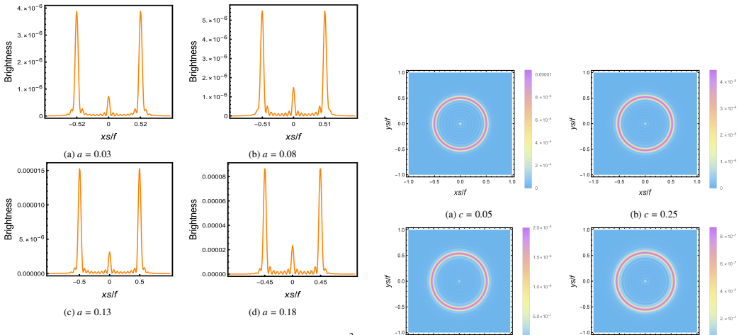
On its own terms, the paper establishes that the boundary response to a Gaussian wave source located at the South pole is a diffraction pattern whose Fourier transform through a virtual convex lens yields a luminous ring, and that the ring's radius follows the parameter trends just stated. The paper applies this holographic imaging method to the quantum-corrected AdS-Reissner-Nordström solution in Kiselev spacetime. The central quantitative result is Eq. (28), $r_R/f = L/\omega^*$, which equates the wave-optics ring angle with the incident angle of photons on the photon sphere, and the authors verify this equality numerically for varying $a$, $c$, and $\Omega$.
Load-bearing premise
The numerical solution of the radial scalar wave equation obtained with the pseudo-spectral method is accurate at the chosen parameter values, because the paper reports no resolution, convergence, or error checks.
Editorial extensions
If this is right
- An observer positioned at the AdS boundary's North pole sees a full axisymmetric ring; moving the observer toward $\theta_{\rm obs} = \pi/2$ turns the image into an arc and finally a point.
- Increasing the quantum-correction parameter $a$, $\Omega$, $T$, or $\mu$ shrinks the ring, while increasing the cosmological-fluid parameter $c$ enlarges it, giving distinct signatures for each parameter.
- Higher wave-source frequency $\omega$ makes the primary ring sharper and suppresses the additional diffraction fringes, so higher-frequency probes yield cleaner radius measurements.
- Across the tested values of $a$, $c$, and $\Omega$, the photon-ring incident angle from geometric optics agrees with the wave-optics ring angle, supporting the correspondence between the two descriptions.
Reading between the lines
- The paper does not prove Eq. (28) as a general identity; it is checked numerically for selected parameters. A natural test is to push the comparison to larger charges, different $\Omega$, and non-Gaussian sources to see whether the match persists.
- If the monotonic trends are robust, the ring radius could serve as a holographic observable to constrain the quantum-correction scale and the Kiselev fluid parameters from synthetic black hole images.
- Because the analysis fixes the source at the South pole and scans only the observer angle, a non-axisymmetric source or off-polar observation could reveal whether the extracted radius is a property of the spacetime or of the imaging geometry.
Editorial analysis
A structured set of objections, weighed in public.
Referee Report
Summary. The manuscript applies the standard AdS/CFT holographic-imaging construction to a quantum-corrected AdS-Reissner-Nordström black hole in Kiselev spacetime. It solves the radial Klein-Gordon equation numerically, extracts the boundary response to a Gaussian source, images the response through a convex lens, and compares the resulting Einstein-ring radius with the geometric-optics photon incident angle. The central quantitative claims are that the ring radius decreases with increasing a, Ω, T, and μ, increases with c, and sharpens with increasing ω, and that the wave-optics ring angle agrees with the photon-ring angle via r_R/f = L/ω*.
Significance. If established, the paper would extend holographic Einstein-ring studies to a new parameterized family of charged, quantum-corrected AdS spacetimes and would provide a non-trivial test of the geometric-optics correspondence for that family. The use of the established dictionary from Hashimoto et al. and Liu et al. is appropriate, and the comparison in Eq. (28) is a falsifiable consistency check. However, the paper's quantitative conclusions are currently undermined by internal inconsistencies in the metric function and by confounded parameter scans.
major comments (4)
- [Section 2, Eq. (4)] The transformation from Eq. (2) to Eq. (4) is inconsistent: with r=1/y and F(y)=y^2 f(1/y), the Reissner-Nordström term Q^2/r^2 becomes Q^2 y^4, not Q^2 y^2 as printed. This affects the horizon condition, the temperature, and every subsequent numerical result. In fact, the temperature values reported in Fig. 17 (e.g., T=0.3918 for Q=0.1, yh=5) are reproduced only if F contains Q^2 y^4 and T is computed as -F'(yh)/(4π), whereas the text states T = F'(yh)/(4π). The manuscript is therefore internally inconsistent and not reproducible as written.
- [Section 3.2, Figs. 17-20] The temperature and chemical-potential scans do not isolate the stated variable. In the temperature scan (Figs. 17-18), yh=5 is fixed and Q takes values 0.1, 0.12, 0.14, 0.16; since μ=yhQ, μ varies from 0.5 to 0.8, contradicting the stated fixed μ=0.5. In the chemical-potential scan (Figs. 19-20), yh=5 is fixed and Q takes values 0.0196, 0.0556, 0.0835, 0.1022; these give μ roughly 0.098, 0.278, 0.418, 0.511 rather than the claimed 0.1, 0.3, 0.5, 0.7, and the temperature varies from about 0.487 to 0.387 rather than being fixed at 0.5 (using the corrected F). Hence the claimed separate dependences of the ring radius on T and on μ are confounded with changes in Q and with each other, and the abstract's central claim about these dependences is unsupported.
- [Section 2, numerical method] The pseudo-spectral solution of Eq. (14) is presented without any resolution, convergence, or error estimates. The extracted ring radii in Section 3 are reported to two decimal places, but there is no evidence that the truncation error is below this precision. Because every quantitative claim depends on these numerical solutions, the accuracy premise must be established, for example by showing convergence with grid size and consistency checks against known limits.
- [Section 4, Figs. 22-24] The geometric-optics comparison in Figs. 22-24 labels the left and right columns as fixing μ=0.5 or T=0.5, but the manuscript does not state the corresponding values of Q and yh for these runs. In light of the inconsistencies in Section 3.2, it is unclear whether the parameter choices actually satisfy the stated constraints, so the comparison is not reproducible as presented.
minor comments (6)
- [Fig. 20 caption] In the Fig. 20 caption, 'ω = −2/3' should read 'Ω = −2/3', and the value of the frequency ω (stated in the text as 90) is missing; the caption also misspells 'brightness' as 'brigheness'.
- [Eqs. (10), (16), (17)] The notation for the response function is inconsistent: Eq. (10) defines ⟨K⟩_{JK}, while Eqs. (16) and (17) use ⟨K⟩^{JK}_l and ⟨K⟩^{JK}; please unify the notation.
- [After Eq. (16)] The sentence 'Therefore, in Eq.(14), ⟨K⟩^{JK}_l can be replaced by ⟨K⟩_l' appears to refer to Eq. (16), not Eq. (14).
- [Eqs. (24) and (25)] In Eqs. (24) and (25), the expressions 'cosθ2_in' and 'sinθ2_in' should be cos^2 θ_in and sin^2 θ_in.
- [Section 3 heading] The Section 3 heading has a stray comma: 'The formation of Einstein ring,'.
- [Throughout] The paper contains numerous typographical errors, including 'di fferent' for 'different' and 'vaules' for 'values' in the Fig. 19 caption; a careful proofread is needed.
Circularity Check
No significant circularity: the Einstein-ring radius from wave optics and the photon incident angle from geometric optics are computed independently and compared as a consistency check, not as a fitted identity.
full rationale
The paper's central derivation chain is: (i) the quantum-corrected AdS-Reissner-Nordstrom metric in Kiselev spacetime is taken from the literature (Eq. 2, from ref. [50]); (ii) the massless scalar field response function is obtained by solving the Klein-Gordon equation (Eqs. 5-16) using the standard holographic dictionary of refs. [30,31,33]; (iii) the Einstein ring is formed by applying the virtual lens setup of ref. [33] (Eqs. 18-21); (iv) the geometric photon incident angle is computed independently from null geodesics in the same metric (Eqs. 22-26); and (v) the two are compared via Eq. (28), r_R/f = L/omega*. Nothing in this chain fits a parameter from one side to force agreement with the other: the wave-optics ring radius r_R is read from the screen brightness peaks, while L/omega* is obtained from the photon-sphere conditions dot r = 0 and dz/dr = 0. The numerical agreement could in principle fail, so it is a genuine consistency test. The many self-citations in the reference list are background and not load-bearing for the main comparison, which relies on the well-known frameworks of Hashimoto et al. and Liu et al.; the metric itself is an input from prior independent work. One non-circularity issue should be noted separately: the temperature and chemical-potential scans in Section 3.2 do not hold the conjugate variable fixed. In Fig. 17 the text states a fixed chemical potential mu = 0.5, but yh = 5 with Q = 0.1, 0.12, 0.14, 0.16 gives mu = yh Q = 0.5, 0.6, 0.7, 0.8; similarly the mu scan in Fig. 19 changes Q at fixed yh and does not keep T = 0.5 fixed. This makes those particular trends confounded, but it is a correctness/parameter-isolation flaw, not circularity, and does not affect the independent geometric-optics comparison. Under the stated circularity criteria, the paper earns a score of 0.
Assumptions & free parameters
free parameters (5)
- AdS radius ℓ =
1
- Scalar field mass M^2 =
-2
- Gaussian source width η =
0.02
- Convex lens radius d =
0.6
- Baseline spacetime parameters (a, c, Ω, Q, e, ω, y_h) =
a=0.1, c=0.1, Ω=-2/3, Q=0.1, e=0.5, ω=90, y_h=5
assumptions (6)
- domain assumption AdS/CFT correspondence (gauge/gravity duality) is valid for this spacetime.
- domain assumption The metric (Eq 2) correctly describes a quantum-corrected AdS-Reissner-Nordstrom black hole in Kiselev spacetime.
- standard math The bulk scalar field obeys the Klein-Gordon equation (Eq 5) with mass M^2=-2 and charge e, and the holographic dictionary gives the response function via Eq (10).
- domain assumption The convex lens transformation (Eq 20), a Fourier transform, correctly converts the boundary response into the screen image.
- standard math The photon ring is determined by the conditions r_dot=0 and dz/dr=0, and the incident angle is given by sin^2 θ_in = L^2/(ω*)^2.
- ad hoc to paper The contribution of the explicit wave source term in Eq (10) is negligible at the observation position.
Cite this review
Pith. "Pith review of Holographic Einstein Ring of Quantum Corrected AdS-Reissner-Nordstrom Black Holes in Kiselev Spacetime." pith.science (2026). https://pith.science/paper/DVRVY64C
@misc{pith2026250115139,
  author       = {Pith},
  title        = {Pith review of: Holographic Einstein Ring of Quantum Corrected AdS-Reissner-Nordstrom Black Holes in Kiselev Spacetime},
  year         = {2026},
  howpublished = {\url{https://pith.science/paper/DVRVY64C}},
  note         = {Machine review of arXiv:2501.15139}
}
abstract
This study, grounded in AdS/CFT correspondence, utilizes wave optics theory to explore the Einstein ring of a quantum-corrected AdS-Reissner-Nordstr\"om black hole (BH) in Kiselev spacetime. By fixing the wave source on the AdS boundary, the corresponding response function generated on the antipodal side of the boundary is successfully obtained. Using a virtual optical system with a convex lens, the holographic image of the Einstein ring of the BH is captured on a screen. The study also investigates the impact of various physical parameters and the observer's position on the characteristics of the Einstein ring. The results indicate that changes in the observer's position cause the image to transition from an axisymmetric ring to an arc, ultimately converging to a single luminous point. Additionally, the Einstein ring radius decreases with increasing values of the quantum correction parameter $a$, the equation of state parameter $\Omega$, temperature $T$, and chemical potential $\mu$ , respectively. In contrast, the ring radius increases as the cosmological fluid parameter $c$ increases. Furthermore, the ring radius becomes more distinct as the wave source frequency $\omega$ increases. From the perspective of geometric optics, the photon ring of the quantum-corrected AdS-Reissner-Nordstr\"om BH in Kiselev spacetime is further studied. Numerical results suggest that the incident angle of the photon ring aligns with that of the Einstein ring.
Figures


Figures from the paper (15 more)







Reference graph
Works this paper leans on
-
[1]
J. M. Maldacena, Adv. Theor. Math. Phys. 2 (1998), 231-252
work page 1998
-
[2]
S. A. Hartnoll, C. P. Herzog and G. T. Horowitz, JHEP 12 (2008), 015
work page 2008
-
[3]
S. A. Hartnoll, C. P. Herzog and G. T. Horowitz, Phys. Rev. Lett. 101 (2008), 031601
work page 2008
-
[4]
S. S. Gubser, Phys. Rev. D 78 (2008), 065034
work page 2008
- [5]
-
[6]
H. Liu, J. McGreevy and D. Vegh, Phys. Rev. D 83 (2011), 065029
work page 2011
-
[7]
T. Faulkner, H. Liu, J. McGreevy and D. Vegh, Phys. Rev. D 83 (2011), 125002
work page 2011
- [8]
Show all 59 references
-
[9]
Kiritsis and J
E. Kiritsis and J. Ren, JHEP 09 (2015), 168
2015
-
[10]
Donos and J
A. Donos and J. P. Gauntlett, JHEP 06 (2014), 007
2014
-
[11]
Shipley and S
J. Shipley and S. R. Dolan, Class. Quant. Grav. 33 (2016) no.17, 175001
2016
-
[12]
Bambi and K
C. Bambi and K. Freese, Phys. Rev. D 79 (2009), 043002
2009
-
[13]
Atamurotov, A
F. Atamurotov, A. Abdujabbarov and B. Ahmedov, Astrophys. Space Sci. 348 (2013), 179-188
2013
-
[14]
A. K. Mishra, S. Chakraborty and S. Sarkar, Phys. Rev. D 99 (2019) no.10, 104080
2019
-
[15]
P. G. Nedkova, V . K. Tinchev and S. S. Yazadjiev, Phys. Rev. D88 (2013) no.12, 124019
2013
-
[16]
Y . X. Chen, H. B. Zheng, K. J. He, G. P. Li and Q. Q. Jiang, Chin. Phys. C 48 (2024), no.12, 125104
2024
-
[17]
K. J. He, Z. Luo, S. Guo and G. P. Li, Chin. Phys. C 48, no.6, 065105 (2024)
2024
-
[18]
Shaikh, P
R. Shaikh, P. Kocherlakota, R. Narayan and P. S. Joshi, Mon. Not. Roy. Astron. Soc. 482 (2019) no.1, 52-64
2019
-
[19]
X. Wang, Z. Zhao, X. X. Zeng and X. Y . Wang, [arXiv:2501.08287 [gr- qc]]
-
[20]
C. Y . Yang, M. I. Aslam, X. X. Zeng and R. Saleem, [arXiv:2411.11807 [astro-ph.HE]]
-
[21]
K. J. He, G. P. Li, C. Y . Yang and X. X. Zeng, [arXiv:2411.11680 [astro- ph.HE]]
-
[22]
K. J. He, J. T. Yao, X. Zhang and X. Li, Phys. Rev. D 109, no.6, 064049 (2024)
2024
-
[23]
K. J. He, S. C. Tan and G. P. Li, Eur. Phys. J. C 82, no.1, 81 (2022)
2022
-
[24]
K. J. He, X. Zhang and X. Li, Chin. Phys. C 46, no.7, 075103 (2022)
2022
-
[25]
K. J. He, S. Guo, S. C. Tan and G. P. Li, Chin. Phys. C 46, no.8, 085106 (2022)
2022
-
[26]
X. X. Zeng, G. P. Li and K. J. He, Nucl. Phys. B 974, 115639 (2022)
2022
-
[27]
K. J. He, C. Y . Yang and X. X. Zeng, [arXiv:2501.06778 [astro-ph.HE]]
-
[28]
Akiyama et al
K. Akiyama et al. [Event Horizon Telescope], Astrophys. J. Lett. 875 (2019), L1
2019
-
[29]
Akiyama et al
K. Akiyama et al. [Event Horizon Telescope], Astrophys. J. Lett. 930 (2022) no.2, L12
2022
-
[30]
Hashimoto, S
K. Hashimoto, S. Kinoshita and K. Murata, Phys. Rev. Lett. 123 (2019) no.3, 031602
2019
-
[31]
Hashimoto, S
K. Hashimoto, S. Kinoshita and K. Murata, Phys. Rev. D 101 (2020) no.6, 066018
2020
-
[32]
Y . Kaku, K. Murata and J. Tsujimura, JHEP 09 (2021), 138 11
2021
-
[33]
Y . Liu, Q. Chen, X. X. Zeng, H. Zhang, W. L. Zhang and W. Zhang, JHEP 10 (2022), 189
2022
-
[34]
X. X. Zeng, K. J. He, J. Pu, G. p. Li and Q. Q. Jiang, Eur. Phys. J. C 83 (2023) no.10, 897
2023
-
[35]
X. X. Zeng, L. F. Li and P. Xu, Eur. Phys. J. C 84 (2024) no.7, 714
2024
-
[36]
X. X. Zeng, M. I. Aslam, R. Saleem and X. Y . Hu, [arXiv:2311.04680 [gr-qc]]
-
[37]
X. Y . Hu, X. X. Zeng, L. F. Li and P. Xu, Results Phys.61 (2024), 107707
2024
-
[38]
G. P. Li, K. J. He, X. Y . Hu and Q. Q. Jiang, Front. Phys. (Beijing) 19 (2024), no.5, 54202
2024
-
[39]
K. J. He, Y . W. Han and G. P. Li, Phys. Dark Univ.44 (2024), 101468
2024
-
[40]
Z. Luo, K. J. He and J. Li, [arXiv:2409.11885 [gr-qc]]
-
[41]
X. X. Zeng, L. F. Li, P. Li, B. Liang and P. Xu, Sci. China Phys. Mech. Astron. 68 (2025) no.2, 220412
2025
-
[42]
X. X. Zeng, X. Y . Hu and K. J. He, [arXiv:2406.03083 [hep-th]]
-
[43]
J. Y . Gui, X. X. Zeng, K. J. He and H. Ye, [arXiv:2407.09069 [hep-th]]
-
[44]
K. J. He, Y . W. Han and G. P. Li, Nucl. Phys. B1010, 116768 (2025)
2025
-
[45]
D. I. Kazakov and S. N. Solodukhin, Nucl. Phys. B 429 (1994), 153-176
1994
-
[46]
R. A. Konoplya, Phys. Lett. B 804 (2020), 135363
2020
-
[47]
C. Liu, T. Zhu, Q. Wu, K. Jusufi, M. Jamil, M. Azreg-A¨ınou and A. Wang, Phys. Rev. D101 (2020) no.8, 084001 [erratum: Phys. Rev. D103 (2021) no.8, 089902]
2020
-
[48]
V . B. Bezerra, I. P. Lobo, J. P. Morais Grac ¸a and L. C. N. Santos, Eur. Phys. J. C 79 (2019) no.11, 949
2019
-
[49]
Shahjalal, Nucl
M. Shahjalal, Nucl. Phys. B 940 (2019), 63-77
2019
-
[50]
J. P. Morais Grac ¸a, E. Folco Capossoli, H. Boschi-Filho and I. P. Lobo, Phys. Rev. D 107 (2023) no.2, 024045
2023
-
[51]
Sadeghi, S
J. Sadeghi, S. Noori Gashti, M. R. Alipour and M. A. S. Afshar, Chin. Phys. C 48 (2024) no.11, 115115
2024
-
[52]
V . V . Kiselev, Class. Quant. Grav.20 (2003), 1187-1198
2003
-
[53]
A. S. Khan and F. Ali, Phys. Dark Univ. 26 (2019), 100389
2019
-
[54]
L. G. C. Gentile, P. A. Grassi and A. Mezzalira, JHEP 10 (2013), 065
2013
-
[55]
Dunn and C
J. Dunn and C. Warnick, Class. Quant. Grav. 33 (2016) no.12, 125010
2016
-
[56]
T. K. Dey, Int. J. Mod. Phys. A 33 (2018) no.33, 1850193
2018
-
[57]
Banerjee, A
N. Banerjee, A. Bhattacharjee and A. Mitra, JHEP 01 (2021), 038
2021
-
[58]
M. R. Khosravipoor and M. Farhoudi, Eur. Phys. J. C 83 (2023) no.11, 1045
2023
-
[59]
I. R. Klebanov and E. Witten, Nucl. Phys. B 556 (1999), 89-114 12
1999
Reviewed August 10, 2026 · model on record in the stance chip above.
Discussion (0). Continue with ORCID to comment.