REVIEW 3 major objections 5 minor 1 cited by
No Equations Needed: Learning System Dynamics Without Relying on Closed-Form ODEs
T0 review · 3 major / 5 minor · reviewed 2026-08-09 · deepseek-v4-flash
Pith's one-line read This paper argues that dynamical systems can be modeled by predicting their behavior description directly from data, bypassing closed-form ODE discovery and analysis entirely.
desk verdict Genuinely new direct-semantic-modeling idea with real experimental value, but the central exactness guarantee is conditional on an unreported C2-fallback rate and needs to be fixed before publication. read the letter →
The pith
A machine-rendered reading of the paper's core claim, the machinery that carries it, and where it could break.
The reading
What carries the argument
The central machinery is the motif-based semantic representation: ten motifs defined by monotonicity (increasing/decreasing), convexity (convex/concave), and domain type (bounded, unbounded with horizontal asymptote, unbounded diverging), which encode the shape of a trajectory on intervals. A composition is the shortest sequence of motifs covering a trajectory, with transition points marking changes between motifs; properties are numeric descriptors such as transition-point coordinates, derivatives at endpoints, asymptote height, and half-life. Semantic ODE's semantic predictor combines a composition map (a piecewise constant function over initial conditions) with property maps (univariate functions learned per composition), and the trajectory predictor reconstructs a $C^{2}$ trajectory by parametrizing cubic splines through their piecewise-linear second derivative and fitting unbounded parts with purpose-built parametrizations (e.g., logistic-like functions for asymptotic decay). This separation is what makes the semantic representation directly inspectable and editable.
What would settle it
Train Semantic ODE on trajectories of x(t) = sin(t) and ask it to predict beyond the training interval: because the model only emits finite motif compositions, it cannot represent the infinite alternating motif sequence, so extrapolation will not oscillate, which would settle that the representability claim fails for periodic systems.
Extended reading notes
Core claim
The central discovery is that the semantic representation of a dynamical system—its shape in terms of motifs, transition points, derivatives, and asymptotic properties—can be generated directly from data, eliminating the need for post-hoc mathematical analysis of a discovered equation. In Semantic ODE, the semantic predictor Fsem outputs a composition (a sequence of motifs such as increasing-convex, decreasing-convex with horizontal asymptote) and a set of properties (transition-point coordinates, derivatives, asymptote height, half-life), and the trajectory predictor Ftraj converts that representation into a twice-differentiable trajectory. Because the model is built as F = Ftraj ∘ Fsem, the semantic predictor is exactly the semantic representation of the model: no separate analysis step is required. The paper shows that this design supports semantic inductive biases, direct editing of behavior (e.g., forcing an asymptote to zero), and competitive or better prediction accuracy compared to SINDy, WSINDy, PySR, Neural ODE, Neural Laplace, and DeepONet across several low-dimensional systems, including a pharmacokinetic model with only one observed dimension.
Load-bearing premise
The load-bearing premise is that the fixed library of ten motifs and finite compositions is expressive enough to cover the target system's behavior; oscillatory, periodic, or chaotic trajectories have infinite compositions and cannot be predicted beyond the observed time domain.
Editorial extensions
If this is right
- If the central claim is correct, users can specify inductive biases about behavior (e.g., 'the last motif must be decreasing with a horizontal asymptote') directly in the model, instead of choosing equation libraries and sparsity penalties.
- Models can be edited after fitting by constraining a property (for example, setting the horizontal asymptote to zero), and the paper shows this can drastically improve extrapolation error on unseen time domains.
- Semantic ODE can fit trajectories governed by general differential equations, delay differential equations, integro-differential equations, and multi-dimensional systems where only one dimension is observed—settings where closed-form ODE discovery typically struggles.
- The composition map can act as an interpretable description of how trajectory shape changes with initial conditions, including where bifurcations occur in the qualitative behavior.
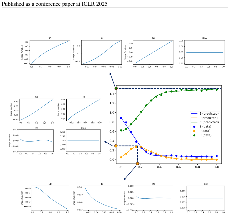
- The authors propose a roadmap for extending direct semantic modeling to multi-dimensional systems using modular per-dimension composition and property maps, with a proof-of-concept on an SIR epidemiological model.
Reading between the lines
- The composition/property split suggests a natural scientific interface: a researcher could hypothesize a behavioral constraint (e.g., 'the peak rises linearly with the dose'), impose it by editing or regularizing the property map, and immediately see the effect—something symbolic-regression pipelines cannot offer without re-deriving the equation.
- If Semantic ODE scales to multiple dimensions, it could make pharmacokinetic and epidemiological models auditable by clinicians and biologists without mathematical training, but only for systems whose behavior is finitely describable; periodic and chaotic dynamics would require an extension to meta-motifs that compress infinite motif sequences.
- Because the semantic representation is the training target rather than a post-hoc summary, one could, in principle, train directly on partial or sparse observations by matching predicted semantic properties, potentially improving sample efficiency in regimes where dense trajectory measurements are unavailable.
- The paper's own limitation—oscillatory, periodic, and chaotic systems have infinite compositions—implies that the method's generality is bounded by the finiteness of the motif sequence; lifting this bound would be the natural next step for real-world cyclic phenomena.
Editorial analysis
A structured set of objections, weighed in public.
Referee Report
Summary. The paper argues that the goal of closed-form ODE discovery is ultimately to obtain a semantic description of the system's behavior, and proposes to predict that semantic description directly from data, bypassing the discover-then-analyze pipeline. It formalizes a semantic representation as a finite composition of ten motifs plus quantitative properties (Section 4), and instantiates the idea in Semantic ODE for 1D systems: a semantic predictor Fsem outputs a composition and a property map, and a trajectory predictor Ftraj reconstructs a trajectory with that semantic representation, so that F = Ftraj ∘ Fsem. The paper presents experiments on synthetic and real datasets showing competitive accuracy, semantic inductive biases, direct editing of the model, and robustness to noise.
Significance. If the guarantee that Fsem equals the semantic representation of the realized model held unconditionally, the paper would be a significant conceptual contribution: it replaces the two-step discover-then-analyze pipeline with a directly inspectable and editable model, and the experiments (Tables 2 and 3) demonstrate practical viability on several non-trivial systems (pharmacokinetic model, DDE, integro-DE, and real datasets). The paper includes machine-checkable proofs of the trajectory-predictor conformity results (Theorems 1 and 2), a representation theorem (Theorem 3), and publicly available code, which are genuine strengths that support reproducibility. However, the conformity guarantee is conditional on the success of the C2 trajectory predictor (with an unmeasured fallback rate), and the representable class is limited to trajectories with finite compositions; these issues temper the significance of the central transparency claim until they are addressed.
major comments (3)
- [Section 5 and Section 5.2.1] The claim that 'by definition, the semantic predictor is the semantic representation of F' holds only when F2_traj succeeds. Section 5.2.1 states that if the L-BFGS-B/Powell optimization does not find a solution with transition-point error below the user-defined threshold, the method 'defaults to F0_traj', whose output is only C0 and, per Appendix D.1.2, may use straight lines between inflection points that are not motifs in the defined set. Thus the realized F = Ftraj ∘ Fsem is not guaranteed to satisfy (cF(x0), pF(x0)) = Fsem(x0) for those inputs, and the semantic representation displayed by Fsem may not describe the trajectory actually generated. The paper reports no statistics on how often F2_traj succeeds or falls back, so the load-bearing transparency guarantee is not verified. Please report fallback rates per dataset and either make Ftraj always return a conforming trajectory or state the guarantee as conditional and characterize when it holds.
- [Appendix G.1 and Theorem 3] Theorem 3 establishes representability only for C2 functions whose second derivative vanishes at finitely many points; oscillatory, periodic, and chaotic trajectories are explicitly outside this class, as Appendix G.1 concedes. Since the title and abstract claim a general approach to 'learning system dynamics', the finite-composition restriction is a substantial scope limitation that should be stated in the abstract and introduction, not only in the supplementary discussion. As presented, the evaluation contains only one non-oscillatory 1D benchmark with an unbounded time domain (logistic growth), with oscillatory systems treated only via bounded-time fitting (Appendix B.6), which is insufficient to support the unqualified claim that direct semantic modeling replaces closed-form ODE discovery for low-dimensional systems.
- [Appendix D.1.2 and Theorem 2] The proof of Theorem 2 uses a relaxed notion of conformity that permits straight-line segments between inflection points, and Lemma 2 requires that the 'other' derivative at the last transition point automatically matches the property in p| because F0_traj is used during training of Fsem. This makes the conformity guarantee for F0_traj an artifact of the training procedure rather than a property of the trajectory predictor alone; if F2_traj falls back to F0_traj at inference on inputs that differ from the training distribution, even that relaxed conformity is not assured. The paper should state this limitation explicitly and provide an inference-time check of conformity whenever F0_traj is used.
minor comments (5)
- [Appendix D.2.2] The heading 's−−b' in the parametrization subsection should be 's−−u', since the surrounding equations (e.g., Eq. (57)) describe an unbounded motif.
- [Section 6.2 and Table 2] Table 2 reports 'out-domain (t>1)' without defining the split in the caption; please state that the out-domain evaluation is on the time interval (1, 2] after scaling, as described in Appendix E.1.
- [Section 5.1] The notation F^{(s++b,s+−h)}_{prop} is difficult to read; consider using a table or a more compact subscript scheme for composition-specific property sub-maps.
- [Figure 10] The loss values in the colorbar of Figure 10 are hard to read and the split points of the composition map are not marked; please add annotations or a clearer color scale.
- [Abstract and Section 1] The abstract says 'low-dimensional dynamical systems' but the implementation is restricted to one-dimensional trajectories; please state this restriction explicitly in the abstract and the introduction so that readers are not misled.
Circularity Check
The direct semantic modeling guarantee is definitional, but the benchmark evaluations and representability proofs are self-contained.
-
self definitional
[Section 5, paragraph after the definition of Ftraj]
"Crucially, by definition, the semantic predictor is the semantic representation of F. Indeed, let x = F (x0) = Ftraj(Fsem(x0)). Then by the definition of Ftraj above, (CF , PF )(x0) = (cF (x0), pF (x0)) = (cx, px) = Fsem(x0)."
F is defined as Ftraj composed with Fsem, and Ftraj is defined as a map that returns a trajectory whose semantic representation equals its input (c, p). Therefore the identity (CF, PF) = Fsem follows immediately from the definitions, not from any empirical discovery or fitted result. The paper uses this identity as the core justification that direct semantic modeling 'eliminates the need for post-hoc mathematical analysis.' That justification is a design tautology: the model is constructed so that its semantic representation is exactly what Fsem outputs. This does not undermine the external benchmark results, which are measured on held-out trajectories, but the 'semantic predictor is the semantic representation' claim is true by construction rather than by validation.
full rationale
The only notable circularity is the definitional guarantee in Section 5 that the semantic predictor equals the semantic representation of the forecasting model. Because F = Ftraj ∘ Fsem and Ftraj is required to return a trajectory conforming exactly to the requested (c, p), the equality (CF, PF) = Fsem is a direct consequence of the architecture's definitions. This is a self-definitional design property, and the paper labels it as such ('by definition'), rather than presenting it as an empirical result. The load-bearing empirical claims are not circular: forecasting errors are computed on held-out trajectories from known generating systems, including ODEs, delay differential equations, and integro-differential equations, and the comparison protocols in Section 6 and Appendix E are standard train/validation/test splits. The representability theorem in Appendix G.5 is a self-contained mathematical proof for C2 functions with finitely many second-derivative zeros; it does not rely on fitted values or self-citations. The references to the authors' prior motif framework are not load-bearing because the motifs used in this paper are redefined in Definition 4, and the paper's extension to unbounded motifs and horizontal asymptotes is its own construction. The fallback from F2_traj to F0_traj and the relaxed conformity in Appendix D.1.2 are internal consistency and robustness issues, not circularity, since the paper's conformity guarantees are stated with those relaxations. Overall, the central benchmarking and mathematical claims are self-contained; the score reflects the one design tautology that is explicit but not empirically validated.
Assumptions & free parameters
free parameters (6)
- Composition library size =
Up to 3 motifs (logistic growth: up to 2)
- Maximum number of composition branches I =
3 in all experiments
- Property-map basis-function weights =
Learned, values not reported
- Composition map split points and branch assignments =
Learned, values not reported
- Unbounded motif parameterization coefficients =
Derived from fitted properties and endpoint derivatives
- Trajectory predictor thresholds and penalties =
0.001 tolerance; derivative penalty terms
assumptions (6)
- domain assumption Trajectories are twice continuously differentiable and have finitely many zeros of the second derivative
- domain assumption The fixed set of ten motifs is sufficient to represent the behavior of the systems studied
- standard math Initial value problems have unique solutions under stated regularity conditions
- ad hoc to paper The trajectory predictor can always find a conforming trajectory within tolerance
- domain assumption Property maps vary smoothly with the initial condition, so extrapolation over x0 is valid
- domain assumption Compared equation discovery baselines are representative and were tuned fairly
invented entities (2)
-
Motif-based semantic representation (ten motifs, compositions, transition points, unbounded-motif properties)
-
Semantic ODE framework (Fsem, Ftraj, composition map, property maps)
Cite this review
Pith. "Pith review of No Equations Needed: Learning System Dynamics Without Relying on Closed-Form ODEs." pith.science (2026). https://pith.science/paper/XUASO3R3
@misc{pith2026250118563,
  author       = {Pith},
  title        = {Pith review of: No Equations Needed: Learning System Dynamics Without Relying on Closed-Form ODEs},
  year         = {2026},
  howpublished = {\url{https://pith.science/paper/XUASO3R3}},
  note         = {Machine review of arXiv:2501.18563}
}
read the original abstract
Data-driven modeling of dynamical systems is a crucial area of machine learning. In many scenarios, a thorough understanding of the model's behavior becomes essential for practical applications. For instance, understanding the behavior of a pharmacokinetic model, constructed as part of drug development, may allow us to both verify its biological plausibility (e.g., the drug concentration curve is non-negative and decays to zero) and to design dosing guidelines. Discovery of closed-form ordinary differential equations (ODEs) can be employed to obtain such insights by finding a compact mathematical equation and then analyzing it (a two-step approach). However, its widespread use is currently hindered because the analysis process may be time-consuming, requiring substantial mathematical expertise, or even impossible if the equation is too complex. Moreover, if the found equation's behavior does not satisfy the requirements, editing it or influencing the discovery algorithms to rectify it is challenging as the link between the symbolic form of an ODE and its behavior can be elusive. This paper proposes a conceptual shift to modeling low-dimensional dynamical systems by departing from the traditional two-step modeling process. Instead of first discovering a closed-form equation and then analyzing it, our approach, direct semantic modeling, predicts the semantic representation of the dynamical system (i.e., description of its behavior) directly from data, bypassing the need for complex post-hoc analysis. This direct approach also allows the incorporation of intuitive inductive biases into the optimization algorithm and editing the model's behavior directly, ensuring that the model meets the desired specifications. Our approach not only simplifies the modeling pipeline but also enhances the transparency and flexibility of the resulting models compared to traditional closed-form ODEs.
Figures


Figures from the paper (13 more)




Forward citations
Cited by 1 Pith paper
-
Beyond the ATE: Interpretable Modelling of Treatment Effects over Dose and Time
SemanticATE models average treatment effects as smooth, interpretable surfaces over dose and time, using surrogate outcomes and a dose-driven semantic trajectory model.
Reference graph
Works this paper leans on
-
[1]
Appendix A: notation and definitions
-
[2]
Appendix B: additional results
-
[3]
Appendix C: training of the semantic predictor
-
[4]
Appendix D: trajectory predictor
-
[5]
Appendix E: experimental details
-
[6]
Appendix F: extended related works
-
[7]
Appendix G: additional discussion A N OTATION AND DEFINITIONS A.1 N OTATION Symbols used throughout this work can be found in Tables 4 and 5. A.2 D EFINITIONS In this section, we provide formal definition of some of the terms introduced in the main text. From the work by Kacprzyk et al. (2024b). Definition 3. Let I be a set of intervals on R and let F be ...
work page 2024
-
[10]
As u| needs to pass through both (0, u0) and (t1, u1) and needs to have ˙u|(0) = u′ 0, we get the following equations. β0 = u0 (11) β3t3 1 + β2t2 1 + β1t1 + β0 = u1 (12) β1 = u′ 0 (13) As in Table 9, we denote u(t1)−u(t0) t1−t0 as κ. Then u1 = u0 + κ × t1. The second equation then reduces to β3t2 1 + β2t1 + u′ 0 = κ (14) Now we have to go by all six cases...
work page 2025
Show all 16 references
-
[11]
asymptotic doubling time
+ u′ 0 = κ (25) By rearranging, we get β3 = u′ 0 − 2κ t2 1 (26) β2 = 3κ − 2u′ 0 t1 (27) To satisfy the conditions of Theorem 1, we need to ensure that ¨u|(t) < 0 for all t ∈ (0, t1). That is we need 6 u′ 0 − 2κ t2 1 t + 23κ − 2u′ 0 t1 < 0 (28) which is equivalent to (6u′ 0 − 1...
2025
-
[12]
half-life
= 0 (68) as required. If there is no bounded motif before it, there is no way to set the second derivative at tend to any other value than 0. This property is fixed and not trained in the property map. Let γ(t) be defined as earlier, i.e., γ(t) = |x(2t) − |x(t) (69) We can com...
2011
-
[15]
In the WSINDy variant, we choose the maximum number of terms during hyperparameter tuning (between 1 and 20)
WSINDy-5 enforces the maximum number of terms to be 5 which would hopefully allow for analyzing the equation. In the WSINDy variant, we choose the maximum number of terms during hyperparameter tuning (between 1 and 20). For both WSINDy and WSINDy-5, we tune the parameter α of ...
2024
-
[24]
Finally, we add a Gaussian noise with a standard deviation σ = 0.01 for the low noise setting and σ = 0.2 for the high noise setting
Then we scale the dataset by dividing the concentrations by 20 and the time points by 24. Finally, we add a Gaussian noise with a standard deviation σ = 0.01 for the low noise setting and σ = 0.2 for the high noise setting. The out-domain dataset is created similarly, but each...
2025
-
[50]
We then solve the initial value problem to obtain a trajectory for each
We create 200 samples of x0 equally spaced between −3 and 3. We then solve the initial value problem to obtain a trajectory for each. We observe each trajectory at 20 equally spaced time points between 0 and 5. Then we scale the dataset by dividing x by 3 and the time points b...
1977
-
[2016]
11 Published as a conference paper at ICLR 2025 Ricky T
ISBN 978-1-119-12150-3. 11 Published as a conference paper at ICLR 2025 Ricky T. Q. Chen, Yulia Rubanova, Jesse Bettencourt, and David K Duvenaud. Neural Ordinary Differential Equations. In Advances in Neural Information Processing Systems, volume 31. Curran Associates, Inc., ...
2025
-
[2017]
frequency
are concerned with the trajectory’s shape, they are usually aimed at finding subsequences of a time series that represent the most important or repeating patterns. There are also numerous other nonsymbolic time series representation techniques ranging from Piecewise Aggregate ...
2000
-
[2020]
doi: 10.1103/PhysRevE.101.010203
ISSN 2470-0045, 2470-0053. doi: 10.1103/PhysRevE.101.010203. Samuel H. Rudy, Steven L. Brunton, Joshua L. Proctor, and J. Nathan Kutz. Data-driven discovery of partial differential equations. Science Advances, 3(4):e1602614, April 2017. ISSN 2375-2548. doi: 10.1126/sciadv.1602...
Reviewed August 9, 2026 · model on record in the stance chip above.
Discussion (0). Continue with ORCID to comment.