REVIEW 4 major objections 4 minor 55 references
chebgreen: Learning and Interpolating Continuous Empirical Green's Functions from Data
T0 review · 4 major / 4 minor · reviewed 2026-08-09 · deepseek-v4-flash
Pith's one-line read This paper establishes that learned continuous Green's functions for unknown one-dimensional linear operators can be interpolated to unseen control-parameter values with test errors under about 3 percent, including for non-self-adjoint…
desk verdict Genuine continuous extension of EGF interpolation with public code and a real error analysis, but the unseen-parameter claim needs an inconsistency fixed and a check on the injectivity radius before it fully lands. read the letter →
The pith
A machine-rendered reading of the paper's core claim, the machinery that carries it, and where it could break.
The reading
What carries the argument
The load-bearing object is the singular value expansion of the learned Green's function, $G_\theta(x,s) = U(s;\theta)\Sigma(\theta)V^*(x;\theta)$, where $U$ and $V$ are quasimatrices, meaning matrices whose columns are $L^2$ functions represented as Chebyshev interpolants, built by a two-dimensional Chebyshev factorization. Around this object the algorithm constructs an infinite-dimensional analogue of the Stiefel manifold, the space of quasimatrices with orthonormal columns. The essential mechanism is tangent-space interpolation: project each model's singular-function quasimatrix onto the tangent space at a reference parameter, interpolate those tangent points and the singular values with Lagrange polynomials, and retract via quasimatrix QR factorization. The paper supplies the projection formula and proves that it is orthogonal, and its error analysis identifies the QR retraction as the dominant error source.
What would settle it
Learn Green's functions for $d^2u/dx^2 + \theta^2 u = f$ at $\theta=4.9$ and $\theta=5.1$, where the paper shows the first two singular functions swap order, interpolate to $\theta^*=5.0$ with the paper's Algorithm 2, and compare against a directly learned target at 5.0; a test error far above the roughly 3 percent seen in the paper's Airy experiments would show that the sign- and order-corrected tangent-space interpolation does not track the crossing.
Extended reading notes
Core claim
The central discovery claimed is that a continuous empirical Green's function comes with a manifold-interpolation rule that lets it travel in parameter space: the singular functions of the learned Green's function for each sampled parameter $\theta_j$ are treated as points on the Stiefel manifold of quasimatrices, lifted to the tangent space at a reference parameter $\theta_0$ by the projection $\Psi \mapsto \Psi - \Phi\,\mathrm{sym}(\Phi^*\Psi)$, interpolated with Lagrange polynomials, and mapped back by quasimatrix QR factorization, while the singular values are interpolated separately. The paper proves that this projection is the orthogonal projection onto the tangent space, gives error bounds of cubic order for the projection and quadratic order for the QR retraction, and handles mode swaps and sign flips by matching inner products against the reference basis. In the paper's account the result is high-fidelity interpolation for the Poisson, advection-diffusion, Airy, and fractional-Laplacian operators, including extrapolation to $\theta=9$ from models at 6, 7, and 8, with the continuous Chebyshev representation making the pipeline independent of any particular spatial mesh.
Load-bearing premise
The argument assumes that the left and right singular functions of the Green's function vary smoothly enough across the sampled parameter values for Lagrange interpolation inside a single tangent space to represent the unseen parameter, and the paper's error analysis establishes this only asymptotically as the parameter gap goes to zero rather than at the tested gaps such as Airy $\theta$ from 1 to 10.
Editorial extensions
If this is right
- For one-dimensional linear operators with a scalar parameter, the pipeline yields a continuously queryable Green's function from about 100 force-response pairs without writing down the governing equation.
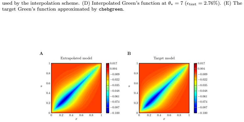
- Interpolated test errors are 0.54 percent for advection-diffusion at $\theta=2.5$, 2.76 percent for Airy at $\theta=7$, and 0.99 percent for the fractional Laplacian at $\theta=0.85$; extrapolation to Airy $\theta=9$ gives 2.28 percent.
- The method extends to non-self-adjoint and nonlocal operators, going beyond the self-adjoint case treated in the prior discrete empirical-Green's-function work.
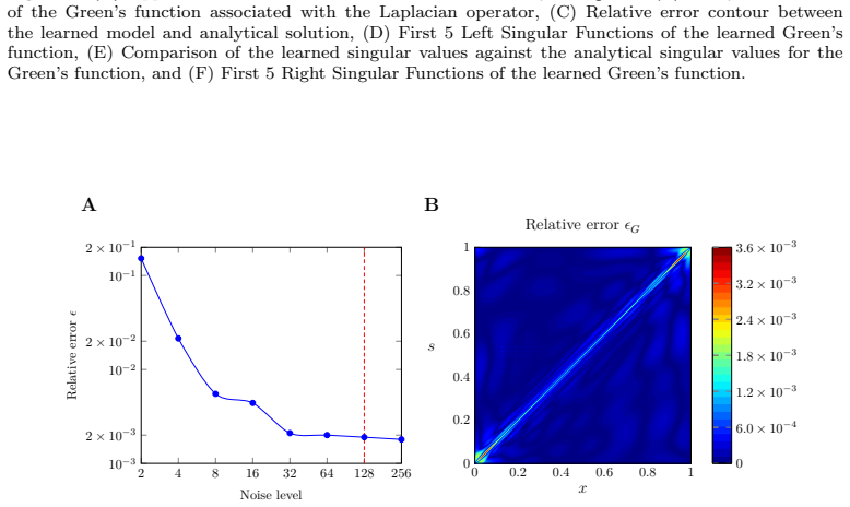
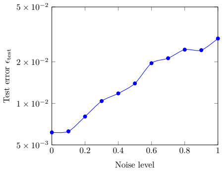
- Training with 50 percent output noise leaves interpolated test errors below about 3.3 percent on the three benchmarks, and the advection-diffusion test error stays below 5 percent even at 100 percent noise.
- Because the representation lives in a Chebyshev basis rather than on a fixed sensor grid, the stored Green's function can be evaluated at arbitrary locations and kept to high precision.
Reading between the lines
- Stress-test extension: interpolate across the singular-value crossing that the paper identifies for the Helmholtz operator at $\theta_{\mathrm{crit}}=\sqrt{5/2}\,\pi$; if the test error spikes at the crossing, the mode-matching assumption, rather than the manifold geometry, is the bottleneck.
- Extension to real sensor data: because the singular value expansion is continuous, the pipeline should in principle accept force-response measurements taken at different sensor locations for different parameter values without first resampling to a common grid; the paper allows arbitrary sensor locations but does not demonstrate this cross-parameter mismatch.
- Higher-dimensional extension: the same tangent-space interpolation would have to be retried on tensor decompositions such as chebfun3/Tucker or tensor-train forms, and the Eckart-Young-Mirsky obstruction the paper flags suggests a different low-rank manifold will be needed there.
Editorial analysis
A structured set of objections, weighed in public.
Referee Report
Summary. The manuscript presents chebgreen, a Python library that learns continuous approximations of Green's functions of one-dimensional linear PDEs from input-output data and interpolates them to new values of a control parameter. The pipeline trains rational neural networks to represent the Green's function and homogeneous solution, converts the learned bivariate function into a Chebyshev-based singular value expansion using a new Python implementation of chebfun, and interpolates the resulting quasimatrices on the tangent space of an infinite-dimensional Stiefel manifold. Numerical experiments cover Poisson, advection-diffusion, Airy, and fractional Laplacian problems, with and without noise; the reported test errors for interpolated models are below about 3%.
Significance. If the results hold, the paper offers a meaningful step beyond the discrete empirical Green's function interpolation of Praveen et al. [32]: the representation is continuous and mesh-independent, it applies to non-self-adjoint operators, and the code is publicly available. The paper also provides a rare external check: for the advection-diffusion case the interpolated Green's function is compared to an analytical expression with relative error 0.26%. The theoretical error analysis (cubic projection error, quadratic retraction error) is elegant but only local; the main support for the central claim is the empirical test-error evidence, which is reasonably strong for the Airy and advection-diffusion experiments.
major comments (4)
- [Section 3.3, Lemma 1] The combined error analysis is asymptotic and local, and the paper does not verify the conditions under which the bounds hold at the parameter spacings used in the experiments. In particular, Lemma 1 guarantees the exponential map is a local diffeomorphism only inside a geodesic ball of radius π, but the manuscript never checks that the learned singular quasimatrices at θ1=1 and θ3=10 in the Airy example lie within that ball around the reference θ0=5. Please either add a numerical check (e.g., compute the norm of the lifted tangent vectors ΓU_j and ΓV_j, or approximate the geodesic distances, and compare with π) or explicitly state that the theoretical bounds are asymptotic and do not cover the finite parameter gaps used in the experiments.
- [Section 4.4] The fractional Laplacian experiment is internally inconsistent: the text states 'interpolating to θ* = 0.9', but θ2 = 0.9 is one of the three training nodes, while the Fig. 16 caption reports 'Interpolated Green's function at θ* = 0.85'. Since the central claim concerns interpolation to unseen parameters, this example must be corrected and re-run; if the intended target is 0.85, the text and Table 1 should be updated consistently.
- [Section 4.2] The advection-diffusion experiment reports Ntrain = 237 input-output pairs, which conflicts with the default Nsamples = 100 (95% training) described in Section 4 and with the sample-size study in Section 4.1.1 that motivates using 100 samples. Please clarify the data budget for this experiment and reconcile the 'order of magnitude lower data' claim with the actual numbers.
- [Section 3.3] The theoretical error analysis covers only the interpolation steps for a given singular value expansion; it does not include the neural network approximation error or the Chebyshev truncation error. The statement that the quadratic retraction error 'dominates the error of the other two steps' is also not a complete error bound for the full pipeline. Please state clearly which sources of error are covered by the theory and which are only assessed empirically.
minor comments (4)
- [Equation (19)] The periodic boundary condition is written as u(−π/2) = u(−π/2) on both sides; it should presumably be u(−π/2) = u(π/2).
- [Algorithm 2, Step 3.2] The notation 'using {[ΓU_j, ΓU_j]}' appears to have a typo; the second entry should likely be ΓV_j.
- [Section 2.7] There is a typo: 'consiedered' should be 'considered'.
- [Section 4.1.1] The x-axis of Fig. 10A is labeled 'Noise level' but the study in Section 4.1.1 is about sample count; please ensure the figure labels match the discussion.
Circularity Check
No load-bearing circularity: the interpolation claim is tested against separately trained target models and one analytical Green's function; the only construction-level problem is the fractional-Laplacian demo, where the text interpolates to a training node (θ*=0.9=θ2), making that 'interpolated' model equal the trained model by construction, while the Fig. 16 caption reports θ*=0.85.
-
self definitional
[Section 4.4 (Fractional Laplacian), text vs. Fig. 16 caption; Algorithm 2 Step 3.2]
"We follow the same procedure of approximating three Green’s functions at parameter values θ1 = 0.8, θ2 = 0.9, and θ3 = 0.95 and interpolating to θ∗ = 0.9. ... (Fig. 16 caption: 'Interpolated Green’s function at θ∗ = 0.85 ϵtest = 0.99%')"
If the text is taken literally, the claimed 'unseen' target θ*=0.9 is exactly the training node θ2=0.9. In Algorithm 2 the base point is the closest node (θ0=θ2), the tangent-space lift of the base point is Γ=U(θ0)−U(θ0)sym(U*(θ0)U(θ0))=0, and Lagrange interpolation evaluated at a node returns that node's value by construction. Hence the 'interpolated' U(0.9), Σ(0.9), V(0.9) coincide with the trained model at θ2, so the reported ϵtest=0.99% merely re-measures the θ2 training model (Table 1 lists 0.95% for θ2) and no unseen parameter is tested. The Fig. 16 caption contradicts the text, so as written one of the three demonstrations reduces to a training input rather than a prediction.
full rationale
The central derivation is self-contained and not circular. The Green's function is learned from forcing–response pairs with rational neural networks [31] and validated externally: the Laplacian model against the analytical Green's function (ϵ=0.36%) and the interpolated advection–diffusion model against the closed-form solution (ϵ=0.26%). The manifold interpolation of Algorithm 2 is tested at genuinely unseen parameters in two demonstrations — Airy θ*=7 with interpolants at θ=1,5,10 and advection–diffusion θ*=2.5 with interpolants at θ=1,2,3 — where the target models are trained on data at θ* that are never used by the interpolation, so those checks are independent and the reported errors (2.76% and 0.54%) are not forced by construction. Citations to the authors' own prior work are routine and not load-bearing: [32] is a published, externally validated method that this paper extends with new proofs (Theorem 1, Propositions 1–2, Lemmas 1–2), and the external inputs to those proofs (Zimmermann–Stoye, Harms–Mennucci, Altmann et al.) are independent literature, not author-derived uniqueness theorems. The paper even candidly admits the gap in its theoretical support — 'no attention has been given to quantifying the size of the region about a base point by which these methods are valid' (Section 3) — which is an honest correctness risk (the injectivity radius π of Lemma 1 is never checked against the finite parameter separations used), but it is not circularity, since the paper presents asymptotic bounds rather than claiming a finite-gap theorem. The single construction-level defect is the fractional-Laplacian demonstration: the text says θ*=0.9, a training node where Lagrange interpolation returns the node's trained SVE by definition, while the figure caption says θ*=0.85; the paper must correct this inconsistency before that demonstration can count as interpolation to an unseen parameter. Because two of the three demonstrations plus the analytical comparison remain independent, the central claim does not reduce to its inputs; the score of 3 reflects one internally inconsistent demonstration and the acknowledged, non-circular limitation in the radius quantification, not load-bearing self-citation.
Assumptions & free parameters
free parameters (4)
- GP length scale sigma =
0.01
- Number of training samples Ntrain =
100 (default), 237 (advection-diffusion)
- Chebyshev tolerance epsilon_cheb =
2.22e-16 (most), 1e-9 (fractional Laplacian)
- Neural network architecture =
4 layers, 50 neurons each
assumptions (5)
- standard math Hilbert-Schmidt theorem ensures a square-integrable Green's function admits an SVE
- standard math Eckart-Young-Mirsky theorem gives optimality of the truncated SVE
- domain assumption Quasimatrix QR factorization is a retraction on the infinite-dimensional Stiefel manifold
- domain assumption Rational NN approximation property from Boulle et al. [31]
- domain assumption The forcing ensemble from a GP with squared-exponential kernel adequately spans the operator's range
Cite this review
Pith. "Pith review of chebgreen: Learning and Interpolating Continuous Empirical Green's Functions from Data." pith.science (2026). https://pith.science/paper/ZTAPL7SY
@misc{pith2026250118715,
  author       = {Pith},
  title        = {Pith review of: chebgreen: Learning and Interpolating Continuous Empirical Green's Functions from Data},
  year         = {2026},
  howpublished = {\url{https://pith.science/paper/ZTAPL7SY}},
  note         = {Machine review of arXiv:2501.18715}
}
read the original abstract
In this work, we present a mesh-independent, data-driven library, chebgreen, to mathematically model one-dimensional systems, possessing an associated control parameter, and whose governing partial differential equation is unknown. The proposed method learns an Empirical Green's Function for the associated, but hidden, boundary value problem, in the form of a Rational Neural Network from which we subsequently construct a bivariate representation in a Chebyshev basis. We uncover the Green's function, at an unseen control parameter value, by interpolating the left and right singular functions within a suitable library, expressed as points on a manifold of Quasimatrices, while the associated singular values are interpolated with Lagrange polynomials.
Figures


Figures from the paper (13 more)







Reference graph
Works this paper leans on
-
[32]
H. Praveen, N. Boull´ e, C. Earls, Principled interpolation of green’s functions learned from data, Computer Methods in Applied Mechanics and Engineering 409 (2023) 115971. doi:10.1016/J.CMA.2023.115971
-
[1]
R. P. Feynman, The Character of Physical Laws, M.I.T. Press, 1967
work page 1967
-
[2]
Raissi, Deep hidden physics models: Deep learning of nonlinear partial differential equations, J
M. Raissi, Deep hidden physics models: Deep learning of nonlinear partial differential equations, J. Mach. Learn. Res. 19 (1) (2018) 932–955
work page 2018
- [3]
-
[4]
J. Berg, K. Nystr¨ om, Neural network augmented inverse problems for PDEs, arXiv preprint arXiv:1712.09685 (2017)
arXiv 2017
-
[5]
L. Lu, X. Meng, Z. Mao, G. E. Karniadakis, Deepxde: A deep learning library for solving differential equations, SIAM Review 63 (2021) 208–228
work page 2021
-
[6]
J. Sirignano, K. Spiliopoulos, Dgm: A deep learning algorithm for solving partial differential equa- tions, Journal of Computational Physics 375 (2018) 1339–1364. doi:10.1016/J.JCP.2018.08.029
- [7]
Show all 55 references
-
[8]
Raissi, P
M. Raissi, P. Perdikaris, G. E. Karniadakis, Physics-informed neural networks: A deep learning framework for solving forward and inverse problems involving nonlinear partial differential equa- tions, J. Comput. Phys. 378 (2019) 686–707
2019
-
[9]
Schaeffer, Learning partial differential equations via data discovery and sparse optimization, Proc
H. Schaeffer, Learning partial differential equations via data discovery and sparse optimization, Proc. R. Soc. A 473 (2197) (2017) 20160446
2017
-
[10]
S. L. Brunton, J. L. Proctor, J. N. Kutz, Discovering governing equations from data by sparse identification of nonlinear dynamical systems, Proc. Natl. Acad. Sci. U.S.A. 113 (15) (2016) 3932– 3937
2016
-
[11]
Champion, B
K. Champion, B. Lusch, J. N. Kutz, S. L. Brunton, Data-driven discovery of coordinates and governing equations, Proceedings of the National Academy of Sciences of the United States of America 116 (2019) 22445–22451
2019
-
[12]
S. H. Rudy, S. L. Brunton, J. L. Proctor, J. N. Kutz, Data-driven discovery of partial differential equations, Sci. Adv. 3 (4) (2017) e1602614
2017
-
[13]
Bonneville, C
C. Bonneville, C. Earls, Bayesian deep learning for partial differential equation parameter discovery with sparse and noisy data, J. Comput. Phys.: X 16 (2022) 100115
2022
-
[14]
Stephany, C
R. Stephany, C. Earls, PDE-READ: Human-readable partial differential equation discovery using deep learning, Neural Netw. 154 (2022) 360–382
2022
-
[15]
Stephany, C
R. Stephany, C. Earls, Pde-learn: Using deep learning to discover partial differential equations from noisy, limited data, Neural Networks 174 (2024) 106242
2024
-
[16]
Stephany, C
R. Stephany, C. Earls, Weak-pde-learn: A weak form based approach to discovering pdes from noisy, limited data, Journal of Computational Physics 506 (6 2024)
2024
-
[17]
Boull´ e, A
N. Boull´ e, A. Townsend, A mathematical guide to operator learning, Handbook of Numerical Anal- ysis 25 (2024) 83–125. doi:10.1016/BS.HNA.2024.05.003
2024 doi
-
[18]
L. Lu, P. Jin, G. Pang, Z. Zhang, G. E. Karniadakis, Learning nonlinear operators via deeponet based on the universal approximation theorem of operators, Nature Machine Intelligence 3 (2021) 218–229
2021
-
[19]
Z. Li, N. Kovachki, K. Azizzadenesheli, B. Liu, K. Bhattacharya, A. Stuart, A. Anandkumar, Fourier neural operator for parametric partial differential equations, Advances in Neural Information Processing Systems 33 (2020) 6755–6766
2020
-
[20]
Z. Li, N. Kovachki, K. Azizzadenesheli, B. Liu, K. Bhattacharya, A. Stuart, A. Anandkumar, Neural operator: Graph kernel network for partial differential equations, arXiv preprint arXiv:2003.03485 (3 2020)
2003 arXiv
-
[21]
Z. Li, N. Kovachki, K. Azizzadenesheli, B. Liu, K. Bhattacharya, A. Stuart, A. Anandkumar, Multipole graph neural operator for parametric partial differential equations, Proceedings of the 34th International Conference on Neural Information Processing Systems (2020)
2020
-
[22]
Z. Li, N. Kovachki, C. Choy, Boyi, J. Kossaifi, S. P. Otta, M. A. Nabian, M. Stadler, C. Hundt, , K. Azizzadenesheli, A. Stuart, A. Anandkumar, Geometry-informed neural operator for large- scale 3d pdes, Proceedings of the 37th International Conference on Neural Information Pr...
2023
-
[23]
Evans, Partial differential equations, 2nd Edition, American Mathematical Society, 2010
L. Evans, Partial differential equations, 2nd Edition, American Mathematical Society, 2010
2010
-
[24]
Khanfer, Applied functional analysis, Applied Functional Analysis (2024) 1–367doi:10.1007/978- 1-4612-0821-1/COVER
A. Khanfer, Applied functional analysis, Applied Functional Analysis (2024) 1–367doi:10.1007/978- 1-4612-0821-1/COVER
2024 doi
-
[25]
Fasshauer, M
G. Fasshauer, M. McCourt, Kernel-based Approximation Methods using MATLAB, Vol. 19, WORLD SCIENTIFIC, 2015. doi:10.1142/9335. 31
2015 doi
-
[26]
Boull´ e, A
N. Boull´ e, A. Townsend, Learning elliptic partial differential equations with randomized linear algebra, Found. Comput. Math. (2022) 1–31
2022
-
[27]
Boulle, A
N. Boulle, A. Townsend, A generalization of the randomized singular value decomposition, in: International Conference on Learning Representations, 2022
2022
-
[28]
Boull´ e, S
N. Boull´ e, S. Kim, T. Shi, A. Townsend, Learning green’s functions associated with time- dependent partial differential equations, The Journal of Machine Learning Research 23 (2022) 1–34. doi:10.5555/3586589.3586807
2022
-
[29]
C. R. Gin, D. E. Shea, S. L. Brunton, J. N. Kutz, DeepGreen: Deep learning of Green’s functions for nonlinear boundary value problems, Sci. Rep. 11 (1) (2021) 1–14
2021
-
[30]
Boulle, Y
N. Boulle, Y. Nakatsukasa, A. Townsend, Rational neural networks, Advances in Neural Information Processing Systems 33 (2020) 14243–14253
2020
-
[31]
Boull´ e, C
N. Boull´ e, C. J. Earls, A. Townsend, Data-driven discovery of Green’s functions with human- understandable deep learning, Sci. Rep 12 (1) (2022) 1–9
2022
-
[33]
Amsallem, C
D. Amsallem, C. Farhat, Interpolation method for adapting reduced-order models and application to aeroelasticity, AIAA Journal 46 (2008) 1803–1813. doi:10.2514/1.35374. URL https://arc.aiaa.org/doi/abs/10.2514/1.35374
2008 doi
-
[34]
Townsend, L
A. Townsend, L. N. Trefethen, An extension of chebfun to two dimensions, SIAM Journal on Scientific Computing 35 (12 2013). doi:10.1137/130908002
2013 doi
-
[35]
T. A. Driscoll, N. Hale, L. N. Trefethen, Chebfun Guide, Pafnuty Publications, 2014
2014
-
[36]
Z. Li, N. B. Kovachki, K. Azizzadenesheli, B. liu, K. Bhattacharya, A. Stuart, A. Anandkumar, Fourier neural operator for parametric partial differential equations, in: International Conference on Learning Representations, 2021
2021
-
[37]
G. W. Stewart, J. guang. Sun, Matrix perturbation theory, Academic Press, 1990
1990
-
[38]
Sukumar, A
N. Sukumar, A. Srivastava, Exact imposition of boundary conditions with distance functions in physics-informed deep neural networks, Computer Methods in Applied Mechanics and Engineering 389 (2022) 114333. doi:10.1016/J.CMA.2021.114333
2022
-
[39]
V. L. Rvachev, T. I. Sheiko, V. Shapiro, I. Tsukanov, Transfinite interpolation over implicitly defined sets, Computer Aided Geometric Design 18 (2001) 195–220. doi:10.1016/S0167-8396(01)00015-2
2001 doi
-
[40]
Biswas, V
A. Biswas, V. Shapiro, Approximate distance fields with non-vanishing gradients, Graphical Models 66 (2004) 133–159. doi:10.1016/J.GMOD.2004.01.003
2004 doi
-
[41]
S¨ uli, D
E. S¨ uli, D. F. Mayers, An introduction to numerical analysis, An Introduction to Numerical Analysis (8 2003). doi:10.1017/CBO9780511801181
2003 doi
-
[42]
Richardson, Chebpy - a python implementation of chebfun
M. Richardson, Chebpy - a python implementation of chebfun. URL https://github.com/chebpy/chebpy
-
[43]
Altmann, D
R. Altmann, D. Peterseim, T. Stykel, Energy-adaptive riemannian optimization on the stiefel man- ifold (2022). arXiv:2108.09831
2022 arXiv
-
[44]
L. N. Trefethen, Householder triangularization of a quasimatrix, IMA Journal of Numerical Analysis 30 (2010) 887–897. doi:10.1093/IMANUM/DRP018
2010 doi
-
[45]
Absil, R
P.-A. Absil, R. Mahony, R. Sepulchre, Optimization Algorithms on Matrix Manifolds, Princeton University Press, Princeton, NJ, 2008
2008
-
[46]
Sternfels, C
R. Sternfels, C. J. Earls, Reduced-order model tracking and interpolation to solve pde-based bayesian inverse problems, Inverse Problems 29 (7) (2013) 075014
2013
-
[47]
Harms, A
P. Harms, A. C. Mennucci, Geodesics in infinite dimensional stiefel and grassmann manifolds, Comptes Rendus Mathematique 350 (15–16) (2012) 773–776. doi:10.1016/j.crma.2012.08.010
2012 doi
-
[48]
Stoye, R
J. Stoye, R. Zimmermann, On the injectivity radius of the stiefel manifold: Numerical investigations and an explicit construction of a cut point at short distance (2024). arXiv:2403.03782. URL https://arxiv.org/abs/2403.03782
2024 arXiv
-
[49]
Biliotti, Exponential map of a weak riemannian hilbert manifold (2006)
L. Biliotti, Exponential map of a weak riemannian hilbert manifold (2006). arXiv:math/0402207. URL https://arxiv.org/abs/math/0402207
2006 arXiv
-
[50]
Boumal, An introduction to optimization on smooth manifolds, Cambridge University Press, 2023
N. Boumal, An introduction to optimization on smooth manifolds, Cambridge University Press, 2023
2023
-
[51]
L. N. Trefethen, Chapter 13. Equispaced Points, Runge Phenomenon, SIAM, 2019, pp. 95–102. doi:10.1137/1.9781611975949.ch13
2019 doi
-
[52]
Hashemi, L
B. Hashemi, L. N. Trefethen, Chebfun in three dimensions, SIAM Journal on Scientific Computing 39 (2017) C341–C363. doi:10.1137/16M1083803;JOURNAL:JOURNAL:SJOCE3;PAGE:STRING:ARTICLE/CHAPTER. 32
2017 doi
-
[53]
Dolgov, D
S. Dolgov, D. Kressner, C. Str¨ ossner, Functional tucker approximation using cheby- shev interpolation, SIAM Journal on Scientific Computing 43 (2021) A2190–A2210. doi:10.1137/20M1356944;WGROUP:STRING:PUBLICATION. URL /doi/pdf/10.1137/20M1356944?download=true
2021 doi
-
[54]
Gorodetsky, S
A. Gorodetsky, S. Karaman, Y. Marzouk, A continuous analogue of the tensor-train de- composition, Computer Methods in Applied Mechanics and Engineering 347 (2019) 59–84. doi:10.1016/J.CMA.2018.12.015. URL https://www.sciencedirect.com/science/article/abs/pii/S0045782518306133
2019 doi
-
[55]
Brivio, S
S. Brivio, S. Fresca, N. R. Franco, A. Manzoni, Error estimates for pod-dl-roms: a deep learning framework for reduced order modeling of nonlinear parametrized pdes enhanced by proper orthog- onal decomposition, Advances in Computational Mathematics 50 (2024) 1–46. doi:10.1007...
2024 doi
Reviewed August 9, 2026 · model on record in the stance chip above.
Discussion (0). Continue with ORCID to comment.