REVIEW 3 major objections 4 minor 51 references
Polydisperse Formation of Planetesimals: The dust size distribution in clumps
T0 review · 3 major / 4 minor · reviewed 2026-08-09 · deepseek-v4-flash
Pith's one-line read A continuous range of dust sizes changes how the streaming instability builds clumps: weaker density peaks, and a size distribution inside clumps that peaks before the largest grains.
desk verdict The GL quadrature method is a clean, well-validated contribution; the peak-in-size-distribution claim is plausible but rides on a 2D geometry the paper itself flags, so it needs a 3D or stratified check before it becomes a prediction. read the letter →
The pith
A machine-rendered reading of the paper's core claim, the machinery that carries it, and where it could break.
The reading
What carries the argument
The central objects are the polydisperse fluid equations in a shearing box, in which dust is described by a size density $\sigma(a)$ and the gas feels the drag backreaction as an integral over sizes, $\rho_g \boldsymbol{\alpha}_{\mathrm{drag},g}=\int \sigma(a)(\mathbf{u}-\mathbf{v}_g)/\tau_s(a)\,da$. The paper approximates this integral with Gauss-Legendre quadrature in log Stokes-number space, mapping the quadrature nodes to stopping times $\tau_{s,j}$ and redefining the dust-species densities as $\rho_{d,j}=\tfrac12 \ln(\tau_{s,\max}/\tau_{s,\min}) w_j\tau_{s,j}\sigma(\tau_{s,j})$, which makes the continuum limit converge much faster with the number of species than uniform binning. The second piece of machinery is the size-dependent drift velocity itself: because each size has a different drift speed through the gas, the clumps develop filaments ordered by Stokes number along the drift direction, which is what places the largest grains outside the highest-density core and creates the peak in the size distribution.
What would settle it
Run the same polydisperse streaming-instability setup in a three-dimensional stratified shearing box with vertical gravity (self-gravity still off) and measure the size distribution in the densest clump cores; if the largest grains no longer sit just outside the core, the predicted peak disappears and the paper's central claim fails.
Extended reading notes
Core claim
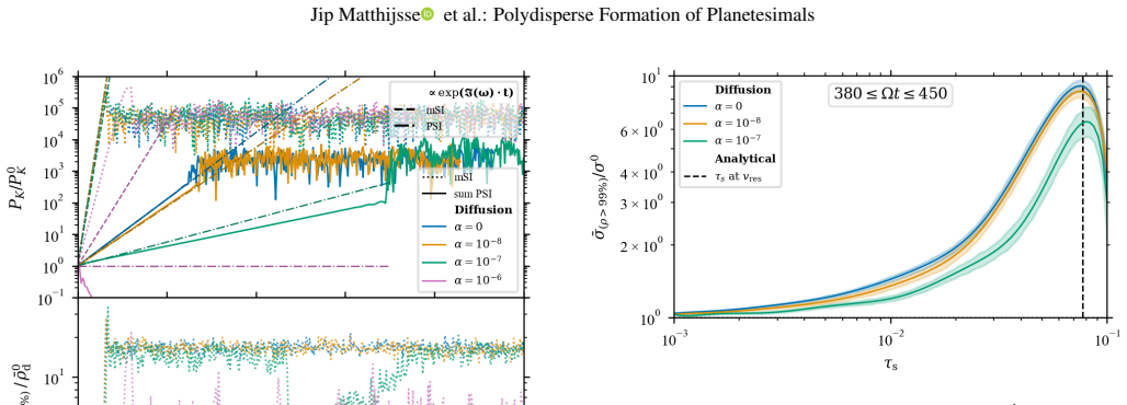
On the paper's own terms, the discovery is that the polydisperse streaming instability behaves qualitatively differently from the monodisperse case in the saturated nonlinear regime, and that the difference leaves a measurable imprint in the dust size distribution of the densest structures. The maximum dust density in the standard polydisperse run is $82\pm 14$ in units of the initial gas density, roughly an order of magnitude below the monodisperse counterpart and below the nominal Roche-density clumping threshold for a low-mass disc; the instability's growth rate is also lower, and it cannot be reproduced by a single-size run with the average Stokes number. Within the densest combined-dust regions, abundances rise with grain size until the largest Stokes numbers, which are spatially segregated just outside the densest core, producing a peak in the size distribution. The same peaked shape is found in individual clumps, across spatial resolutions, dust-species counts, sampling methods, and diffusion coefficients, and also at dust-to-gas ratios of 3 and 1, but not at 0.5 where the instability does not grow.
Load-bearing premise
The whole picture depends on the assumption that a two-dimensional, vertically unstratified, isothermal slice without self-gravity preserves the way dust sizes sort themselves inside clumps, so the same peak would appear in a real three-dimensional disc.
Editorial extensions
If this is right
- Planetesimal formation through the streaming instability needs stronger conditions (higher dust-to-gas ratio or weaker turbulence) than single-size studies suggested, because polydisperse clumps stall below the Roche density in the standard setup.
- Rubble-pile asteroids may carry a size distribution imprinted by instability dynamics rather than by coagulation: a peak at an intermediate size with a deficit of the very largest grains, even if no growth occurred.
- Polydisperse simulations cannot be replaced by monodisperse runs tuned to the average dust size; the average-size run overestimates clumping by roughly a factor of 3.5 in the standard case.
- The faster-converging quadrature sampling makes full size-distribution simulations affordable with only about ten dust species, opening the door to parameter surveys that were previously expensive.
- Because the largest grains are located just outside the densest core, any body that collapses from the core will be depleted in the most weakly coupled sizes relative to the surrounding disc.
Reading between the lines
- A natural but unstated consequence: if the segregation pattern survives in three dimensions, the size distribution of observed rubble-pile asteroids could be used as a probe of the local gas density and turbulence level at the formation site.
- The same size-sorting mechanism might operate in other dusty flows with size-dependent drift (e.g., radial drift in the disc), so the peak-and-deficit pattern could be a general signature of polydisperse drag instabilities, not just the streaming instability.
- The paper's 2D runs cannot settle whether the peak appears in the bodies that actually form; a testable extension is to seed 3D stratified simulations with the same size distribution and check whether the largest grains still segregate out of the core before collapse.
- Because the quadrature treats the dust species as integration nodes rather than physical bins, the method transfers to any code that already evolves multiple pressureless fluids; this suggests a low-cost path for incorporating continuous size distributions into broader disc-evolution models.
Editorial analysis
A structured set of objections, weighed in public.
Referee Report
Summary. The paper studies the polydisperse streaming instability (PSI) in the nonlinear regime using 2D, unstratified, isothermal shearing-box simulations with multiple pressureless dust fluids. It introduces Gauss-Legendre quadrature over Stokes number to discretize the drag back-reaction integral and validates this method against the publicly available psitools linear solver. In the linear regime, the GL method reproduces the analytic growth rate to within about 0.3% with nd=5 and about 0.07% with nd=10, whereas the log-spaced discrete method requires roughly 40 bins for comparable accuracy (Table 2). In the saturated regime, the polydisperse instability reaches maximum dust densities about an order of magnitude below the monodisperse case, and the 99th-percentile size distribution is peaked: larger Stokes numbers are overrepresented in dense structures, except for the largest size, which is spatially offset from the densest part of the combined dust distribution (Secs. 5.1 and 7). The authors attribute this peak to size-dependent spatial segregation and connect it to the dust size distribution that could end up in planetesimals.
Significance. If the results hold, the Gauss-Legendre quadrature scheme is a practical improvement for multispecies streaming-instability simulations, and the paper provides a clean external validation against an independent open-source solver, with openly archived data and analysis code. The linear-regime comparison is the strongest part of the paper and is convincingly quantified; the monodisperse comparisons at both the maximum and the averaged Stokes number are thoughtful controls. The most interesting physical claim, a dynamically produced peak in the size distribution of the densest clumps, is falsifiable and relevant for planetesimal and rubble-pile size distributions. Its robustness is currently limited because the peak and its segregation explanation are demonstrated only within the 2D unstratified model, and the paper itself concedes that a 3D assessment is required; those limitations are openly stated, which is to the authors' credit.
major comments (3)
- [Sec. 7 and Fig. 19] The central claim that spatial segregation causes the peak in the size distribution rests on a qualitative reading of a single snapshot. Figure 19 shows the 99th-percentile contours of four dust bins at Omega t = 166.5, while the peak statistic in Figures 6 and 8 is time-averaged over a saturated interval; the text in Sec. 7 says that the largest Stokes numbers lie 'just outside' the densest regions without quantifying that offset. The alternative resonance explanation is also left unresolved in Sec. 5.1, where the overlap is described as visual and 'does not convincingly correspond' to the peak. To make this load-bearing inference quantitative, the authors should compute a species-resolved segregation diagnostic, such as cross-correlations of density fields or centroid offsets of the high-density regions as a function of Stokes number, over the saturated interval, and show that its time dependence tracks the position and amplitude of the peak.
- [Sec. 5.2.1 and Sec. 8.1] The quantitative statement about maximum dust density is resolution-dependent. The authors correctly state in Sec. 5.2.1 that, without diffusion, the dust fluid does not converge with spatial resolution and that the maximum density increases with resolution; nevertheless Sec. 8.1 quotes rho_d,max = 82 +/- 14 rho0_g as a main result and compares it with the Roche density. Because the 256-1024 grid trend in Figure 7 is not extrapolated or otherwise bounded, the conclusion that PSI clumps fall below the strong-clumping criterion should not be presented as a converged quantitative result. Please report how the 82 +/- 14 value behaves with resolution, or identify a resolution-independent statistic, such as a converged percentile, to support the comparison.
- [Sec. 8.1] The paper's geometry limits the main astrophysical prediction. The authors note that the simulations are 2D unstratified, that 3D simulations are required to assess clumping via the Roche density, that 3D could change the shape of clumps and therefore the spatial separation between dust sizes, and that unstratified linear growth rates are not good predictors of clumping in stratified simulations (Li & Youdin 2021). Since the peaked size distribution in dense regions and its planetesimal-formation relevance depend on this segregation persisting outside the 2D unstratified box, the conclusion should either be explicitly restricted to the 2D model or supported by a 3D or stratified check. A concrete test would be a same-parameter 3D unstratified run, and if feasible a stratified run, measuring whether the Stokes-dependent centroid offset and the resulting peak persist.
minor comments (4)
- [Sec. 3.1] The sentence 'If we want to work in log-size space we can map these notes to the correct Stokes number' should say 'nodes' rather than 'notes'.
- [Sec. 5.2.1] In the final paragraph, 'a weak trend in the position of the peak to drift to smaller stroke numbers' should be 'smaller Stokes numbers'.
- [Fig. 15 caption] The caption for Figure 15 is identical to the caption for Figure 13; if the figure is intended to show the Stokes-range runs discussed in Sec. 6.2, the caption should be corrected accordingly.
- [Sec. 6.4] In the sentence describing the dust-to-gas ratio runs, the color assignment is duplicated ('in green' twice) and there is a missing closing parenthesis after 'run PSI_mu,3'; please check the intended colors against Figure 18.
Circularity Check
No significant circularity: the polydisperse peak and density reductions are measured simulation results, with self-citations used only as benchmarks.
full rationale
The paper's central claims—reduced PSI clumping and the peak in the size distribution at the densest regions—are measured from FARGO3D simulation outputs, not derived from fitted parameters or from the linear theory. The GL quadrature is validated against independently computed psitools linear growth rates; this is a code benchmark, and the nonzero errors in Table 2 show the comparison has discriminative power. Seeding the simulation with the psitools eigenvector tests whether the discrete numerical scheme reproduces the continuum linear operator; it does not encode the nonlinear peak or the maximum dust density. The spatial-segregation explanation is inferred from density contours of individual dust species (Fig. 19) and cross-checked with discrete sampling and clump-averaged size distributions, so it is not equivalent by construction to the 99th-percentile diagnostic. Self-citations to psitools and to Paardekooper & Aly (in prep.) are contextual or benchmark references, not load-bearing premises for the new results. Concerns about the 2D unstratified geometry affecting the peak are external-validity limitations that the paper itself concedes, and they are not a form of circularity.
Assumptions & free parameters
free parameters (3)
- Upper Stokes number tau_s,max =
0.1 Omega^-1 (standard), also 0.05 and 0.2
- Power-law slope beta of the size distribution =
-3.5 (MRN), also -3.2 and -3.8
- Dust-to-gas ratio mu =
3 (standard), also 0.5 and 1
assumptions (6)
- standard math Gauss-Legendre quadrature accurately approximates the drag integral when the integrand is smooth; verified only in the linear regime for the initial size distribution.
- domain assumption The dust is a pressureless fluid, valid only for Stokes numbers much smaller than 1; this justifies tau_s,max = 0.1.
- domain assumption The unstratified isothermal shearing box with no vertical gravity represents the disc midplane and captures the clumping-relevant physics.
- domain assumption The linear eigenvalue calculations from psitools correctly describe the polydisperse streaming instability in the continuum limit.
- domain assumption The dust size distribution is continuous and follows an MRN power law sigma(a) proportional to a^(3+beta), beta = -3.5.
- ad hoc to paper The spatial segregation of dust species, inferred from a single 2D snapshot, is the cause of the peak in the size distribution.
Cite this review
Pith. "Pith review of Polydisperse Formation of Planetesimals: The dust size distribution in clumps." pith.science (2026). https://pith.science/paper/XZYGIWGU
@misc{pith2026250201752,
  author       = {Pith},
  title        = {Pith review of: Polydisperse Formation of Planetesimals: The dust size distribution in clumps},
  year         = {2026},
  howpublished = {\url{https://pith.science/paper/XZYGIWGU}},
  note         = {Machine review of arXiv:2502.01752}
}
read the original abstract
The streaming instability is an efficient method for overcoming the barriers to planet formation in protoplanetary discs. The streaming instability has been extensively modelled by hydrodynamic simulations of gas and a single dust size. However, more recent studies considering a more realistic case of a particle size distribution show that this will significantly decrease the growth rate of the instability. We follow up on these studies by evaluating the polydisperse streaming instability, looking at the non-linear phase of the instability at the highest density regions, and investigating the dust size distribution in the densest dust structures. We employ 2D hydrodynamic simulations in an unstratified shearing box with multiple dust species representing an underlying continuous dust size spectrum using FARGO3D. To calculate the drag force on the gas due to a continuous dust size distribution, we apply the Gauss-Legendre quadrature method in dust size space. This method converges faster with the number of dust species than the usual uniform sampling method. The polydisperse streaming instability is less efficient than its monodisperse counterpart in generating dense clumps that could collapse into planetesimals. In the densest dust structure, the larger dust sizes are more abundant because they are less coupled to the gas and, therefore, can clump together more than the smaller dust grains. This trend is broken at the largest dust size due to size-dependent spatial segregation of the highest-density regions, where particles with the largest Stokes numbers are located just outside the densest areas of the combined dust species. This is observed as a peak in the size distribution at the densest regions, which could relate to the size distribution that ends up in the planetesimal after collapse and can mimic the size distribution of dust growth.
Figures


Figures from the paper (14 more)




Reference graph
Works this paper leans on
-
[1]
Bai, X.-N. & Stone, J. M. 2010, ApJ, 722, 1437 Benítez-Llambay, P., Krapp, L., & Pessah, M. E. 2019, ApJS, 241, 25 Benítez-Llambay, P. & Masset, F. S. 2016, ApJS, 223, 11
work page 2010
-
[2]
W., & Dullemond, C
Birnstiel, T., Ormel, C. W., & Dullemond, C. P. 2011, A&A, 525, A11
2011
-
[3]
2017, MNRAS, 469, S755
Blum, J., Gundlach, B., Krause, M., et al. 2017, MNRAS, 469, S755
2017
-
[4]
T., Capaccioni, F., Filacchione, G., et al
Capria, M. T., Capaccioni, F., Filacchione, G., et al. 2017, MNRAS, 469, S685
work page 2017
-
[5]
Chapman, C. R. 1978, 2053, 145
work page 1978
-
[6]
Chen, K. & Lin, M.-K. 2020, ApJ, 891, 132 Delft High Performance Computing Centre (DHPC). 2024, DelftBlue Su- percomputer (Phase 2), https://www.tudelft.nl/dhpc/ark:/44463/ DelftBluePhase2
work page 2020
-
[7]
Draine, B. T. & Lee, H. M. 1984, ApJ, 285, 89
1984
-
[8]
Epstein, P. S. 1924, Physical Review, 23, 710
1924
Show all 51 references
-
[9]
& Blum, J
Fulle, M. & Blum, J. 2017, MNRAS, 469, S39
2017
-
[10]
Garaud, P., Barrière-Fouchet, L., & Lin, D. N. C. 2004, ApJ, 603, 292
2004
-
[11]
& Lynden-Bell, D
Goldreich, P. & Lynden-Bell, D. 1965, MNRAS, 130, 125
1965
-
[12]
J., Minton, D
Graves, K. J., Minton, D. A., Molaro, J. L., & Hirabayashi, M. 2019, Icarus, 322, 1
2019
-
[13]
& Blum, J
Gundlach, B. & Blum, J. 2013, Icarus, 223, 479
2013
-
[14]
R., Millman, K
Harris, C. R., Millman, K. J., van der Walt, S. J., et al. 2020, Nature, 585, 357
2020
-
[15]
2022, Nature As- tronomy, 6, 1043
Hsu, H.-W., Wang, X., Carroll, A., Hood, N., & Horányi, M. 2022, Nature As- tronomy, 6, 1043
2022
-
[16]
Hunter, J. D. 2007, Computing in Science and Engineering, 9, 90
2007
-
[17]
2011, MNRAS, 415, 3591
Jacquet, E., Balbus, S., & Latter, H. 2011, MNRAS, 415, 3591
2011
-
[18]
S., Mac Low, M.-M., et al
Johansen, A., Oishi, J. S., Mac Low, M.-M., et al. 2007, Nature, 448, 1022
2007
-
[19]
Krapp, L., Benítez-Llambay, P., Gressel, O., & Pessah, M. E. 2019, ApJ, 878, L30
2019
-
[20]
& Lin, M.-K
Lehmann, M. & Lin, M.-K. 2023, MNRAS, 522, 5892
2023
-
[21]
& Youdin, A
Li, R. & Youdin, A. N. 2021, ApJ, 919, 107
2021
-
[22]
B., Li, R., et al
Lim, J., Simon, J. B., Li, R., et al. 2024b, arXiv e-prints, arXiv:2410.17319
-
[23]
Magnan, N., Heinemann, T., & Latter, H. N. 2024, MNRAS, 529, 688
2024
-
[24]
S., Rumpl, W., & Nordsieck, K
Mathis, J. S., Rumpl, W., & Nordsieck, K. H. 1977, ApJ, 217, 425
1977
-
[25]
P., Lovascio, F., & Paardekooper, S.-J
McNally, C. P., Lovascio, F., & Paardekooper, S.-J. 2021, MNRAS, 502, 1469
2021
-
[26]
G., et al
Mottola, S., Arnold, G., Grothues, H. G., et al. 2015, Science, 349, 2.232
2015
-
[27]
1986, Icarus, 67, 375 Nesvorný, D., Li, R., Youdin, A
Nakagawa, Y ., Sekiya, M., & Hayashi, C. 1986, Icarus, 67, 375 Nesvorný, D., Li, R., Youdin, A. N., Simon, J. B., & Grundy, W. M. 2019, Nature Astronomy, 3, 808
1986
-
[28]
P., & Lovascio, F
Paardekooper, S.-J., McNally, C. P., & Lovascio, F. 2020, MNRAS, 499, 4223
2020
-
[29]
P., & Lovascio, F
Paardekooper, S.-J., McNally, C. P., & Lovascio, F. 2021, MNRAS, 502, 1579
2021
-
[30]
A., Marrocchi, Y ., Morbidelli, A., et al
Pinto, G. A., Marrocchi, Y ., Morbidelli, A., et al. 2021, ApJ, 917, L25
2021
-
[31]
P., et al
Poulet, F., Lucchetti, A., Bibring, J. P., et al. 2016, MNRAS, 462, S23
2016
-
[32]
Rucska, J. J. & Wadsley, J. W. 2023, MNRAS, 526, 1757 Schäfer, U., Johansen, A., & Banerjee, R. 2020, A&A, 635, A190
2023
-
[33]
2021, A&A, 653, A14
Schaffer, N., Johansen, A., & Lambrechts, M. 2021, A&A, 653, A14
2021
-
[34]
2018, A&A, 618, A75
Schaffer, N., Yang, C.-C., & Johansen, A. 2018, A&A, 618, A75
2018
-
[35]
Shakura, N. I. & Sunyaev, R. A. 1973, A&A, 24, 337
1973
-
[36]
B., Blum, J., Birnstiel, T., & Nesvorný, D
Simon, J. B., Blum, J., Birnstiel, T., & Nesvorný, D. 2022, arXiv e-prints, arXiv:2212.04509
2022 arXiv
-
[37]
I., Cuzzi, J
Simon, J. I., Cuzzi, J. N., McCain, K. A., et al. 2018, Earth and Planetary Science Letters, 494, 69
2018
-
[38]
& Hopkins, P
Squire, J. & Hopkins, P. F. 2020, MNRAS, 498, 1239
2020
-
[39]
2005, ApJ, 625, 414
Tanaka, H., Himeno, Y ., & Ida, S. 2005, ApJ, 625, 414
2005
-
[40]
1964, ApJ, 139, 1217
Toomre, A. 1964, ApJ, 139, 1217
1964
-
[41]
M., Estrada, P
Umurhan, O. M., Estrada, P. R., & Cuzzi, J. N. 2020, ApJ, 895, 4
2020
-
[42]
E., et al
Virtanen, P., Gommers, R., Oliphant, T. E., et al. 2020, Nature Methods, 17, 261
2020
-
[43]
G., Dr˛ a˙ zkowska, J., & Dominik, C
Visser, R. G., Dr˛ a˙ zkowska, J., & Dominik, C. 2021, A&A, 647, A126 Wahlberg Jansson, K. & Johansen, A. 2017, MNRAS, 469, S149
2021
-
[44]
Walsh, K. J. 2018, ARA&A, 56, 593
2018
-
[45]
2019, ApJ, 884, 178
Weber, P., Pérez, S., Benítez-Llambay, P., et al. 2019, ApJ, 884, 178
2019
-
[46]
Weidenschilling, S. J. 1977, Ap&SS, 51, 153
1977
-
[47]
2018, ApJ, 868, 27
Yang, C.-C., Mac Low, M.-M., & Johansen, A. 2018, ApJ, 868, 27
2018
-
[48]
& Zhu, Z
Yang, C.-C. & Zhu, Z. 2021, MNRAS, 508, 5538
2021
-
[49]
& Johansen, A
Youdin, A. & Johansen, A. 2007, ApJ, 662, 613
2007
-
[50]
Youdin, A. N. & Goodman, J. 2005, ApJ, 620, 459
2005
-
[51]
& Yang, C.-C
Zhu, Z. & Yang, C.-C. 2021, MNRAS, 501, 467 Article number, page 16 of 16
2021
Reviewed August 9, 2026 · model on record in the stance chip above.
Discussion (0). Continue with ORCID to comment.