REVIEW 3 major objections 4 minor 13 references
An Alternate Method for Minimizing $\chi^2$
T0 review · 3 major / 4 minor · reviewed 2026-08-08 · deepseek-v4-flash
Pith's one-line read This paper introduces SFit, a χ² minimizer that approximates the Hessian with products of first derivatives, and reports that on 1,716 KMTNet microlensing light curves it fits faster than Nelder-Mead and with fewer misleading…
desk verdict A useful microlensing fitting package with a benchmark whose headline claim—'more reliable than BFGS'—doesn't hold up to a fair comparison. read the letter →
The pith
A machine-rendered reading of the paper's core claim, the machinery that carries it, and where it could break.
The reading
What carries the argument
The load-bearing object is the derivative-product approximation in Equation 8, which replaces the true Hessian (the matrix of second derivatives of $\chi^2$) with $-2\sum_k \sigma_k^{-2}\,(\partial F/\partial A_i)(\partial F/\partial A_j)$. This matrix is exactly the Hessian for linear models because the residual-weighted second-derivative term vanishes; the paper keeps the same form for nonlinear models as an approximation. The machinery inverts that approximate Hessian to get a step direction, applies an adaptive step-size multiplier, and reads parameter uncertainties from the diagonal of the inverse matrix. For microlensing, the point-lens model and its derivatives are supplied by the MulensModel package, with the two flux parameters per dataset included as free parameters for SFit but fitted by linear least squares inside each evaluation for the SciPy comparison algorithms.
What would settle it
Re-run the same 1,716-event sample with identical flux-parameter handling for every algorithm—for instance, linear-subtract the flux parameters for SFit too—and compare reported success flags and evaluation counts. If SFit no longer shows a lower false-positive/false-negative total or a speed advantage over BFGS and Nelder-Mead, the paper's central comparison collapses.
Extended reading notes
Core claim
The paper's central claim is that a minimizer based on the approximation $\frac{\partial^2\chi^2}{\partial A_i\partial A_j}\approx -2\sum_k \frac{1}{\sigma_k^2}\frac{\partial F(x_k)}{\partial A_i}\frac{\partial F(x_k)}{\partial A_j}$ can serve as a practical Newton-type method. The step is $\Delta_i=\sum_j C_{ij}D_j$ with $C=B^{-1}$ and $B$ built from those derivative products, and a small adaptive step-size parameter $\epsilon$ controls how far the step is taken. On the paper's benchmark of 1,716 point-lens microlensing events, SFit reports success on 1,425 events and every one of those reports is a true positive, whereas BFGS reaches the best of the four minima on nearly all events but reports failure on 32 percent of fits; Nelder-Mead succeeds on 98 percent of events but needs roughly 2.5 times as many function evaluations; Newton-CG has high rates of both false successes and false failures. The paper therefore concludes that SFit is faster than Nelder-Mead and more reliable than BFGS for this application.
Load-bearing premise
The comparison is fair: SFit fits the brightness-scale and background parameters as free parameters, the SciPy algorithms fit those same parameters with a separate linear fit at every step, and success is defined by reaching the best of the four fits within a $\chi^2$ difference of 1.
Editorial extensions
If this is right
- Point-lens microlensing fits can be run with an algorithm that never reports a false success, eliminating a common source of wasted follow-up effort.
- Users can obtain parameter uncertainties from the same derivative products used for the minimization, with no extra Hessian calculation.
- The benchmark numbers give a concrete cost comparison: median 167 $\chi^2$ evaluations for SFit, 34 for BFGS, and 419 for Nelder-Mead on this sample.
- Failure flags from BFGS and Nelder-Mead should not be read as 'no minimum found,' because most of their reported failures still reach the best minimum.
- Newton-CG should be avoided for this kind of light-curve fitting.
Reading between the lines
- The comparison embeds the flux parameters differently for SFit than for the SciPy algorithms, so the speed and reliability rankings are not yet separated from parameterization; equalizing that treatment would be a direct test of the paper's headline advantage.
- The same derivative-product Hessian approximation could be tried on any least-squares problem where second derivatives are expensive or noisy, but its usefulness likely hinges on how small the neglected residual-weighted term is near the minimum.
- Extending the benchmark to finite-source or binary-lens microlensing models would show whether the fixed grid and adaptive step size remain stable on model surfaces with strong degeneracies.
Editorial analysis
A structured set of objections, weighed in public.
Referee Report
Summary. The paper presents an optimization algorithm for minimizing chi-square in which the Hessian is approximated by products of first derivatives of the model (Eq. 8), following the approach sketched in Gould (2003). The authors implement this as the Python package SFit, apply it to point-lens microlensing light curves, and benchmark it against BFGS, Nelder-Mead, and Newton-CG from SciPy on 1716 KMTNet 2018 events. The paper's central claim is that, for this application, SFit is faster than Nelder-Mead and more reliable than BFGS, while Newton-CG is ineffective. The derivation is standard but clearly presented; the contribution lies in the implementation and the large real-data performance test.
Significance. If the performance comparison were fair, the paper would be a useful contribution to the microlensing fitting toolbox: it provides a public implementation, estimates parameter uncertainties from the approximate Hessian, and tests the method on a large sample of real survey data rather than on synthetic examples. These are genuine strengths. However, the central comparative claim is weakened by the asymmetric benchmark design: the SciPy baselines solve a smaller effective problem than SFit, and the 'reliability' definition is based on the algorithms' own success flags rather than solely on whether the minimum was actually found. As a result, the advertised advantage over BFGS is not established by the reported tests.
major comments (3)
- [Section 4.2, Tables 1 and 2] The benchmark comparison is asymmetric. For the three SciPy algorithms, the flux parameters fS,k and fB,k are removed by an exact linear fit at every iteration, so the optimizer solves a 3-parameter problem in (t0, u0, tE). For SFit, the flux parameters are included as free parameters, making it a (3+2N)-parameter problem where N is the number of datasets. Therefore Table 2's function-evaluation counts compare two different optimization problems and cannot directly support the speed claims, and Table 1's reliability comparisons conflate algorithmic reliability with problem dimensionality. The authors should rerun the comparison with SFit also linear-fitting the flux parameters at each iteration, or with the SciPy algorithms also treating the flux parameters as free parameters, and report both variants.
- [Section 4.3, Table 1, and Section 5] The abstract's claim that SFit is 'more reliable than the BFGS gradient method' is only true under a definition of reliability based on the algorithm's self-reported success flag. Using the paper's own criterion for actually finding the minimum (Delta chi^2 < 1), BFGS reaches the best minimum on 1714 of 1716 events (1172 reported successes plus 542 reported failures), whereas SFit reaches it on 1429 of 1716 events (1425 reported successes plus 4 reported failures). Under the metric that matters to a user, BFGS is more reliable. The claim should be rephrased to 'more reliable success reporting' or the primary reliability metric should be changed to whether the minimum was found, independent of the algorithm's flag.
- [Section 4.3, Table 1] The classification of fits as 'true positives', 'false positives', etc. uses the algorithm's own success flag together with the Delta chi^2 < 1 criterion. Because the success flags of the SciPy algorithms are known to be unreliable in this application (as the paper itself shows, e.g., 542 BFGS failures nevertheless found the minimum), the four-way classification is informative only about flag behavior, not about actual fitting performance. The paper should present the actual success rate (fraction of events with Delta chi^2 < 1 to the best minimum) as the headline reliability metric, with the flag-based classification as a secondary diagnostic.
minor comments (4)
- [Table 2] The header 'Evalutions' should be corrected to 'Evaluations'.
- [Section 4.2] The text states that tol = 1e-5 for all algorithms, but the meaning of tol differs across SciPy methods (e.g., gtol for BFGS, xatol/fatol for Nelder-Mead). Please specify the option passed for each method so the comparison is reproducible.
- [Section 3.1] The adaptive step-size procedure for epsilon is described only qualitatively ('starts at 0.001 and becomes larger as the minimum is approached'). Since this directly affects the number of function evaluations and convergence behavior, please give the update rule or refer to the relevant code lines.
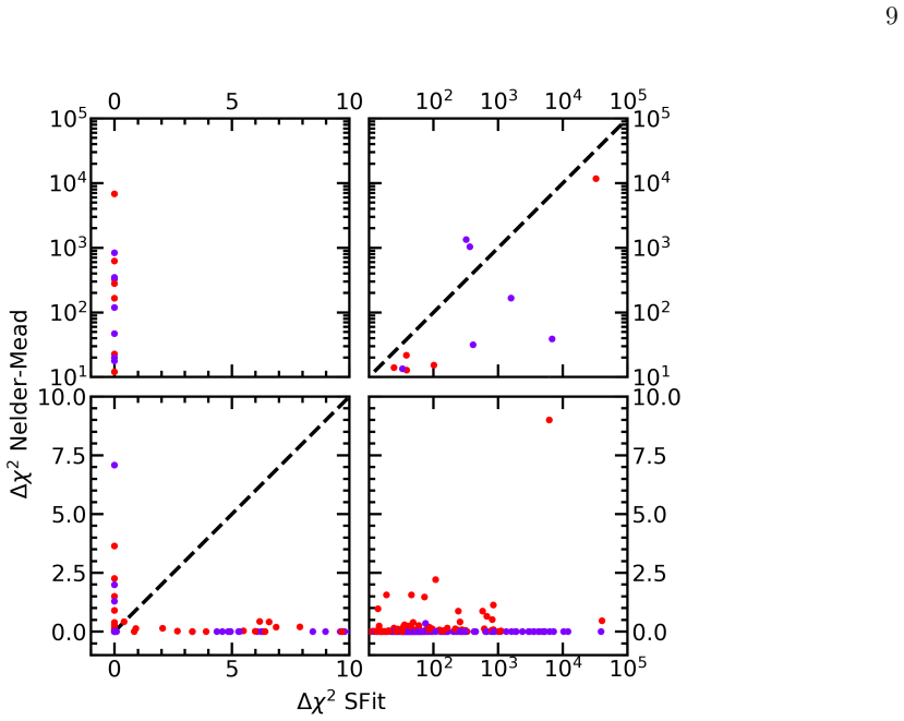
- [Figures 1-3] The captions do not state the color convention (purple = reported success, red = reported failure), although the text refers to these colors. Please add the color legend to the captions.
Circularity Check
No circularity: the derivation is an explicit approximation and performance is benchmarked against independent SciPy implementations.
full rationale
The paper's derivation is self-contained: Section 2 begins with the exact Taylor expansion and exact second derivative (Eqs. 1-6), then explicitly approximates the Hessian by dropping the second-derivative-of-model term (Eq. 8). This is a stated approximation, not an input secretly defined in terms of the output. The algorithm is then tested on 1716 KMTNet events against SciPy's BFGS, Nelder-Mead, and Newton-CG minimizers using public data and independent implementations, so the performance claims are externally benchmarked rather than fitted into existence. The only self-citation is to Gould (2003) as background for the linear-fit special case, but the paper re-derives the equations it uses, making that citation non-load-bearing. The benchmark asymmetry noted by the skeptic (SFit fits flux parameters while the SciPy algorithms linear-fit them at each iteration) is a legitimate fairness concern for the speed/reliability comparison, but it is not a circularity: the comparison is still between the algorithm variants on real data, and no fitted parameter is renamed as a prediction. Thus no circular step can be identified.
Assumptions & free parameters
free parameters (5)
- Adaptive step-size starting value epsilon_0 =
0.001
- Success threshold Delta chi^2 =
1.0
- Maximum chi-square evaluations =
999
- Starter grid for u0 and tE =
u0=[0.01,0.3,0.7,1.0,1.5], tE=[1,3,10,20,40]
- Convergence tolerance tol =
1e-5
assumptions (5)
- domain assumption The second-derivative term containing (y_k - F(x_k)) times d2F/dAi dAj is negligible (Eq. 8).
- domain assumption The best chi-square among the four algorithms is the true minimum for each event.
- ad hoc to paper The differing treatment of flux parameters between SFit and the SciPy methods does not bias the comparison.
- domain assumption KMTNet photometric errorbars are Gaussian after renormalization to chi2/dof = 1.
- domain assumption Derivatives returned by MulensModel are correct and match the implemented chi-square.
Cite this review
Pith. "Pith review of An Alternate Method for Minimizing $\chi^2$." pith.science (2026). https://pith.science/paper/6BNFCZAU
@misc{pith2026250204486,
  author       = {Pith},
  title        = {Pith review of: An Alternate Method for Minimizing $\chi^2$},
  year         = {2026},
  howpublished = {\url{https://pith.science/paper/6BNFCZAU}},
  note         = {Machine review of arXiv:2502.04486}
}
abstract
In this paper, we describe an algorithm and associated software package (sfit_minimize) for maximizing the likelihood function of a set of parameters by minimizing $\chi^2$. The key element of this method is that the algorithm estimates the second derivative of the $\chi^2$ function using first derivatives of the function to be fitted. These same derivatives can also be used to calculate the uncertainties in each parameter. We test this algorithm against several standard minimization algorithms in SciPy.optimize.minimize() by fitting point lens models to light curves from the 2018 Korea Microlensing Telescope Network event database. We show that for fitting microlensing events, SFit works faster than the Nelder-Mead simplex method and is more reliable than the BFGS gradient method; we also find that the Newton-CG method is not effective for fitting microlensing events.
Figures


Reference graph
Works this paper leans on
-
[1]
Albrow, M. D., Horne, K., Bramich, D. M., et al. 2009, MNRAS, 397, 2099, doi: 10.1111/j.1365-2966.2009.15098.x
-
[2]
2012, Computational Optimization and Applications, 51, 259, doi: 10.1007/s10589-010-9329-3
Gao, F., & Han, L. 2012, Computational Optimization and Applications, 51, 259, doi: 10.1007/s10589-010-9329-3
-
[3]
Gaudi, B. S. 2012, ARA&A, 50, 411, doi: 10.1146/annurev-astro-081811-125518
- [4]
-
[5]
2022, A&A, 664, A13, doi: 10.1051/0004-6361/202243744
Gould, A., Han, C., Zang, W., et al. 2022, A&A, 664, A13, doi: 10.1051/0004-6361/202243744
-
[6]
Jung, Y. K., Zang, W., Han, C., et al. 2022, AJ, 164, 262, doi: 10.3847/1538-3881/ac9c5c
-
[7]
Kim, D. J., Kim, H. W., Hwang, K. H., et al. 2018a, AJ, 155, 76, doi: 10.3847/1538-3881/aaa47b
-
[8]
Kim, H.-W., Hwang, K.-H., Kim, D.-J., et al. 2018b, ArXiv e-prints. https://arxiv.org/abs/1804.03352
Show all 13 references
-
[9]
2018c, arXiv e-prints, arXiv:1806.07545
Kim, H.-W., Hwang, K.-H., Shvartzvald, Y., et al. 2018c, arXiv e-prints, arXiv:1806.07545. https://arxiv.org/abs/1806.07545
-
[10]
2016, Journal of Korean Astronomical Society, 49, 37, doi: 10.5303/JKAS.2016.49.1.037 7
Kim, S.-L., Lee, C.-U., Park, B.-G., et al. 2016, Journal of Korean Astronomical Society, 49, 37, doi: 10.5303/JKAS.2016.49.1.037 7
2016 doi
-
[11]
Nocedal, J., & Wright, S. J. 2006, Numerical Optimization (New York, NY: Springer New York), 135–163, doi: 10.1007/978-0-387-40065-5 6
2006 doi
-
[12]
1986, ApJ, 304, 1, doi: 10.1086/164140
Paczynski, B. 1986, ApJ, 304, 1, doi: 10.1086/164140
1986 doi
-
[13]
Poleski, R., & Yee, J. C. 2019, Astronomy and Computing, 26, 35, doi: 10.1016/j.ascom.2018.11.001 8 Figure 1. ∆χ2 of the BFGS model relative to the best-fitting model vs. ∆ χ2 of the SFit model. Fits reported as successes by BFGSare plotted in purple, while those reported as f...
2019 doi
Reviewed August 8, 2026 · model on record in the stance chip above.
Discussion (0). Continue with ORCID to comment.