Deep Learning Models for Physical Layer Communications

Nunzio A. Letizia

REVIEW 4 major objections 4 minor 223 references

Deep Learning Models for Physical Layer Communications

T0 review · 4 major / 4 minor · reviewed 2026-08-08 · deepseek-v4-flash

Challenge this review Re-run · record.json Download PDF Read on arXiv ↗ Review JSON

Pith's one-line read Optimal decoding and capacity-achieving coding can be reformulated as neural estimation problems and learned directly from paired input–output samples, with no tractable channel model required.

desk verdict A coherent, honest compilation of solid but incremental DL-for-comms work; the headline capacity-learning claim is plausible but not established beyond the AWGN benchmark. read the letter →

arxiv 2502.04895 v1 pith:CD6YEMJE submitted 2025-02-07 cs.LG eess.SP

Nunzio A. Letizia This is my paper · ORCID

classification cs.LGeess.SP MSC 94A1794A4068T0762H05

keywords deeplearningphysicallayercommunicationschannelcapacitymutualinformationestimationneuraldecodingautoencodersgenerativeadversarialnetworkscopulas

verification ladder T0 review T1 audit T2 compute T3 formal

The pith

A machine-rendered reading of the paper's core claim, the machinery that carries it, and where it could break.

The reading

This thesis tries to restate the two foundational problems of physical-layer communications — optimal decoding and channel capacity — in the language of machine learning, and to solve them with neural networks trained on paired input–output samples. It claims that no tractable mathematical model of the channel is needed: a discriminative network can learn the a-posteriori probabilities that an optimal decoder needs, and a cooperative generator–discriminator pair can learn the input distribution that achieves capacity. The payoff, if these claims hold, is a data-driven design path for channels where no optimal strategy is known, including power-line and other non-Gaussian media. The argument throughout rests on the same neural machinery: an information-estimation principle that extracts densities and mutual information from the equilibrium of an adversarial value function.

What carries the argument

The central object is the variational representation of the f-divergence, stated as Theorem 3.2.1.1: for convex lower-semicontinuous $f$ with $f(1)=0$ and Fenchel conjugate $f^*$, the divergence between a copula density and the uniform density equals a supremum over functions $T$ of $\mathbb{E}_{c}[T(u)] - \mathbb{E}_{\pi}[f^*(T(u))]$, and the maximizer satisfies $(f^*)'(T(u)) = c(u)$. This identity is the machine that carries the whole argument: it turns density and mutual-information estimation into a trainable adversarial game, and the optimum of that game supplies the density ratio from which the a-posteriori distribution (MIND), the mutual information (f-DIME), and the capacity objective (CORTICAL) are all read off. The copula step — projecting data into the unit cube via their marginal cumulative distributions — is what makes the density ratio well behaved in high dimensions.

What would settle it

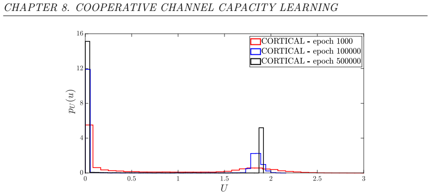
Train CORTICAL on a scalar AWGN channel under a strict peak-power constraint, whose capacity-achieving input distribution is known analytically to be discrete with finite alphabet, and compare the learned input distribution and the estimated capacity to the exact values. A learned distribution that does not converge to the known discrete optimum, or an estimated capacity that exceeds the true channel capacity — impossible for an unbiased estimator at the optimum — would show that the training objective is chasing a biased estimate of mutual information.

Watch

Extended reading notes

Core claim

The central discovery claimed is that mutual information, the quantity whose maximization defines channel capacity and whose minimization defines an optimal decoder, can be turned into a trainable objective. The thesis derives a family of estimators (referred to collectively as f-DIME) from the variational representation of the f-divergence: maximizing a value function built from paired and unpaired samples yields, at equilibrium, the density ratio of paired to product distributions, from which the a-posteriori distribution and the mutual information can be read off. This single device is then used three times: the MIND decoder learns the a-posteriori probability of each codeword given the received signal and decodes by minimizing the resulting a-posteriori information, matching a genie MAP decoder in non-uniform-source, non-linear-channel, and non-Gaussian-noise experiments; the capacity-driven autoencoder adds the estimated mutual information as a regularizer to cross-entropy training to design capacity-approaching codes; and the CORTICAL framework couples a generator that shapes the input distribution with a discriminator that estimates the achieved mutual information, claiming to estimate channel capacity and recover capacity-achieving input distributions in non-Shannon scenarios such as peak-power-limited, non-Gaussian, and fading channels.

Load-bearing premise

The argument rests on the premise that the neural mutual-information estimators are unbiased enough to train against, and that the cooperative generator–discriminator training converges to the true capacity-achieving input distribution, so that optimizing the estimated quantity really optimizes the true one; the thesis validates this against analytically known capacity in only a few figures, not across the claimed generality.

Editorial extensions

If this is right

If the MIND claim holds, receivers for channels with no analytic model — non-linear amplifiers, non-Gaussian noise, unknown source statistics — can be trained from samples, and the same network also returns the achieved information rate and the decoding error probability.
If the capacity-driven autoencoder claim holds, constellation shaping follows the channel's mutual information instead of a hand-picked distance metric, and the reported results show lower block error rates at fixed rate for the tested channels.
If the CORTICAL claim holds, channel capacity becomes a computable number for any discrete-time continuous memoryless vector channel: two cooperating networks return both the capacity estimate and the input distribution that achieves it, matching known results for AWGN and producing new distributions for peak-power-limited, non-Gaussian, and fading channels.
If the f-DIME claim holds, the thesis supplies a family of mutual information estimators with controlled bias and variance, and every decoder, autoencoder, and capacity learner built on them inherits their reliability.

Reading between the lines

Editorial extensions of the paper, not claims the author makes directly.

The density-ratio machinery could be inverted into a model-validation tool: for a proposed parametric channel model, the learned ratio between observed and model-generated outputs should be flat, and any structure would localize exactly where the model fails — a use the thesis does not discuss.
Because the copula step separates dependence from marginals, a copula learned on one medium could plausibly be recombined with the marginals of another, allowing cross-medium channel and noise synthesis without retraining — a transfer possibility the thesis leaves implicit.
A stress test the thesis does not run is distribution-level verification: on a channel whose capacity-achieving input is known analytically and is non-Gaussian, CORTICAL's learned input distribution should match it exactly, not merely produce a capacity number that lands near the true value.

Share X Bluesky LinkedIn Reddit HN

Editorial analysis

A structured set of objections, weighed in public.

Desk editor's note, referee report, and a circularity audit.

Desk Editor's Note

read the letter

Dear colleague,

The one-sentence take: treat this as a polished doctoral thesis that compiles previously published results; the individual pieces are mostly sound and sometimes clever, but the headline claim—capacity learning for arbitrary channels—is not supported by the experiments shown, and I don't think the thesis closes that gap.

What's actually good: MIND is a clean reformulation of MAP decoding as a discriminator that estimates the a-posteriori ratio, and the toy-channel results match the genie MAP decoder; that is a real, useful contribution. The f-DIME family and the derangement sampling trick address a genuine variance problem in neural MI estimation, and the bias/variance tables are a solid piece of empirical work. CODINE's copula-density formulation is also neat and self-consistent. CORTICAL—generator/discriminator cooperative capacity learning—is a plausible idea, and the AWGN peak-power benchmark is the right kind of external check: it recovers a known discrete capacity-achieving distribution, which is non-trivial.

Where it gets soft: the thesis claims capacity estimation and capacity-achieving input distributions for any discrete-time continuous memoryless vector channel. The visible evidence doesn't get there. The f-DIME benchmarks show accurate MI estimation on fixed distributions; that does not imply that maximizing the estimate over a parametric generator family recovers the true capacity-achieving distribution. A small estimator bias can shift the argmax, and the text doesn't analyze that. The CORTICAL sections show learned distributions for AICN and fading channels, but there is no independent optimum to compare against, so the reported capacity is the maximum of the estimator itself. There is also an unresolved representational question: for peak-power AWGN the capacity-achieving input is a discrete PMF, and the text doesn't specify how CORTICAL's continuous generator produces point masses; Fig. 8.2 shows marker radii proportional to PMF, but the mechanism is not explained. These are genuine gaps, not manufactured ones. The reader's report says Ch. 7–8 are missing; they are actually in the text, but they are thin, and the gap analysis above stands.

The thesis is honest about being a compilation; Sec. 1.4 lists the papers, which is good practice. My main caveat is that the abstract and Sec. 1.2 overclaim 'any arbitrary medium.'

Who benefits: grad students and researchers new to DL-for-comms get a readable map of one group's work; MI-estimation people will want the f-DIME chapter. The capacity-learning claim needs more work before it convinces me. I'd send this to serious peer review, but with a clear request to either prove or qualify the argmax/bias issue and to validate on at least one non-Shannon channel with an independent capacity upper bound.

Referee Report

4 major / 4 minor

Summary. This doctoral thesis develops deep-learning methods for physical-layer communications, with contributions in copula-based density estimation (SGN, CODINE), GAN-based channel and noise synthesis, a mutual-information neural decoder (MIND), mutual-information-regularized and capacity-driven autoencoders, a family of f-divergence mutual-information estimators (f-DIME), a cooperative capacity-learning framework (CORTICAL), and applications to power-line communications and trajectory interpolation. The central claims are that MIND achieves the performance of a genie MAP decoder in unknown channels and that CORTICAL estimates channel capacity and learns capacity-achieving input distributions for arbitrary discrete-time continuous memoryless vector channels. The numerical validation visible in the thesis relies mainly on toy channels, comparisons against MAP genie decoders, and closed-form AWGN capacity curves.

Significance. If the capacity-learning claims hold, the thesis would represent a meaningful step toward data-driven physical-layer design for channels without tractable models. The variational derivations for f-DIME and the cooperative CORTICAL training are internally consistent, and the thesis provides useful sanity checks by comparing against known MAP decoding and closed-form AWGN capacity. The presence of machine-checkable code for MIND and CORTICAL and the detailed proofs in Sec. 7.6.2 are additional strengths. However, the significance of the central capacity-learning claim is currently limited because the visible experiments do not validate the method on any non-Shannon channel with an independently known capacity or capacity-achieving distribution.

major comments (4)

[Sec. 8.2] The claim that CORTICAL estimates the channel capacity C = sup_p I(X;Y) rests on three unproven conditions: (i) the f-DIME variational estimate is tight and unbiased, or at least has an argmax that coincides with the true argmax, over the family of generator-induced input distributions; (ii) the parametric generator family can represent the capacity-achieving distribution; and (iii) the cooperative training converges to a global optimum. Sections 7.3-7.6 benchmark f-DIME on fixed distributions, which does not establish that maximizing the estimate over a parametric family preserves the true capacity-achieving distribution. The only quantitative capacity comparisons shown in Sec. 8.3 are against closed-form AWGN capacity. I ask the authors to add at least one non-Shannon validation with an independently known capacity or capacity-achieving distribution, and to report the gap between the f-DIME objective and an independent MI estimate at the learned distribution.
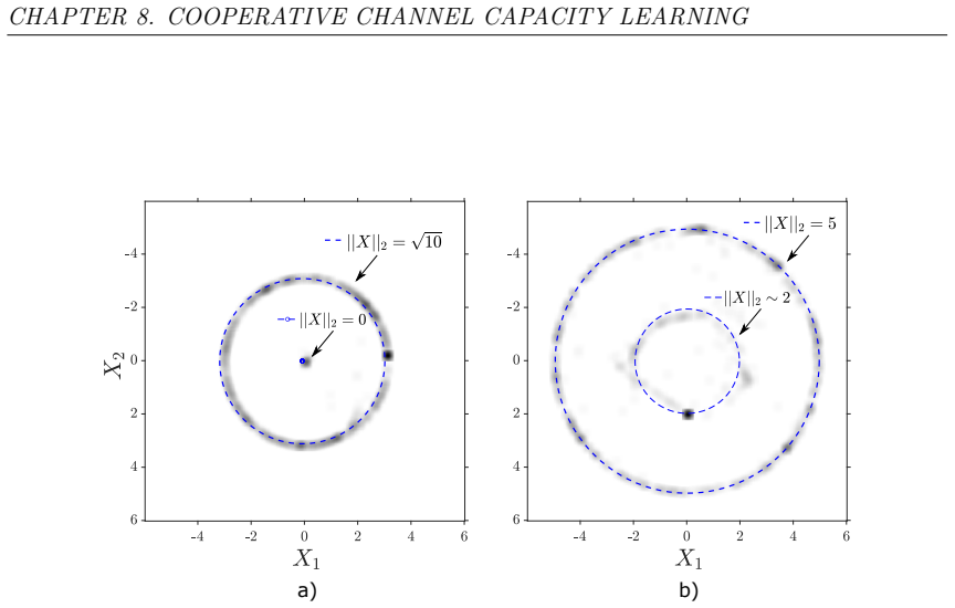
[Sec. 8.3.1, Fig. 8.2] The capacity-achieving input distribution for a peak-power-limited AWGN channel is discrete, with finitely many mass points, but the CORTICAL generator is described as a continuous neural sampler. Figure 8.2 shows markers whose radius is proportional to the PMF, but the text does not specify how a continuous generator output realizes a discrete PMF, for example through output quantization, a Gumbel-softmax relaxation, or convergence to collapsed mixture components. Without this specification, the learned 'distribution' and the reported capacity for this scenario are not well defined. The authors should state the exact generative family and show, analytically or empirically, that it can represent discrete atoms.
[Sec. 6.4] The capacity-driven autoencoder is claimed to construct capacity-approaching codes, but the supporting numerical results in Figs. 6.6-6.10 plot the same neural MI estimator that appears in the training loss. These curves are therefore not independent evidence that the achieved rate approaches the true channel capacity. The authors should compare the learned codes against known capacity or against an independently computed MI for at least one channel, or explicitly frame the results as 'estimated MI achieved by the trained code' rather than as capacity-approaching performance.
[Sec. 5.2.2, Lemma 5.2.2.1] MIND is presented as a general decoding principle, but the decoding rule in Eq. (5.21) requires evaluating the a-posteriori information over all x in the support T_x. For continuous input alphabets this is computationally intractable, and all numerical experiments in Sec. 5.3 use discrete alphabets. The thesis's abstract and Sec. 1.2 claim optimal coding-decoding for arbitrary communication media, but the visible MIND results support only the discrete-input case. The authors should either state this restriction explicitly or provide a tractable decoding procedure for continuous alphabets.

minor comments (4)

[Sec. 5.5.1] The opening sentence of this section says 'we provide extra details on the derivation of the supervised loss function from the supervised one'; this should read 'from the unsupervised one.'
[Sec. 3.2.1, Theorem 3.2.1.1] The theorem assumes f is a convex lower semicontinuous function with f(1)=0 and then uses its derivative f'; please state the additional regularity assumptions needed for the Fenchel-conjugate result and for the pointwise identity c_U(u) = (f^*)'(\hat{T}(u)).
[Abstract and Sec. 1.2] The phrases 'any arbitrary communication medium' and 'for any arbitrary communication medium' are broader than what the visible analysis establishes; the thesis should qualify these statements with the discrete-time, memoryless, stationary assumptions used in Chs. 5-8.
[Chapter 9] The abbreviation list and Chapter 9 use 'Nakagami-m' noise, while the table of contents spells it 'Nagakami-m'; please make the spelling consistent.

Circularity Check

1 steps flagged · score 4.0 of 10

Capacity estimates in Chs. 6 and 8 are, by construction, the maximized values of the same neural MI estimators used as training objectives; external AWGN checks reduce but do not remove this coupling.

fitted input called prediction [Ch. 6 (intro, Sec. 6.3); Ch. 8 (Sec. 8.2)]
"By jointly maximizing the MI and minimizing the cross-entropy, we propose a theoretical approach that a) computes an estimate of the channel capacity and b) constructs an optimal coded signal approaching it. [...] CORTICAL consists of two cooperative networks: a generator with the objective of learning to sample from the capacity-achieving input distribution, and a discriminator with the objective to learn to distinguish between paired and unpaired channel input-output samples. The latter utilizes f-DIME to estimate the MI."

In both schemes, the input distribution labeled capacity-achieving is obtained by gradient ascent on the same neural MI estimate (MINE in Ch. 6, f-DIME in Ch. 8) whose value is then read out as the capacity. The reported number is therefore, by construction, the maximum of the learned estimator over the parametric input family, not an independently measured C = sup_p I(X;Y). Identifying the two requires the estimator to be unbiased and tight at the maximizing distribution and the generator family to contain the true optimum; the visible text does not prove these conditions, and Ch. 7 provides only empirical bias/variance studies on fixed known distributions. The AWGN comparisons in Figs.

full rationale

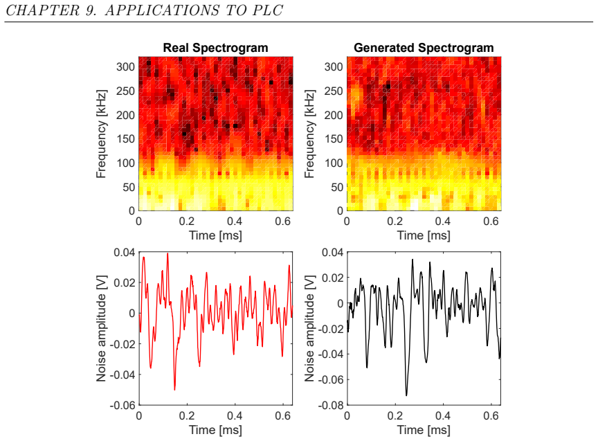
Most of the thesis is self-contained and externally benchmarked: MIND is compared against genie MAP and MaxL decoders on known channels; CODINE is validated on closed-form Gaussian copula densities; channel and noise synthesis is assessed with real PLC measurements; the RST interpolation chapter is checked against minimum-snap and matrix-inversion baselines. These parts do not exhibit circularity. The partial circularity is confined to the capacity-learning claims (capacity-driven AE and CORTICAL). In those chapters, the capacity readout is the value of the MI estimator that also serves as the training reward for the encoder/generator, so the output is fitted to the estimator by construction. The thesis does provide external validation on AWGN channels where closed-form capacity exists, and f-DIME is a genuine variational lower bound with its own synthetic experiments, which prevents a complete reduction to a self-citation or a pure tautology. However, the generalization to arbitrary channels relies on an unproven identification between the maximized estimator output and true capacity, which is a by-construction coupling rather than an independent prediction. Hence a moderate score of 4 is appropriate.

Assumptions & free parameters 3 free parameters · 5 assumptions · 0 invented entities

The thesis introduces new neural architectures and training methods but no new physical entities; the load-bearing assumptions are standard math and domain assumptions about channel stationarity and GAN convergence.

free parameters (3)

beta (MI regularization weight) = 0.2 (in experiments)
Controls trade-off between cross-entropy and mutual information in rate-driven autoencoders; chosen by hand in Sec. 6.3.2.
epsilon (label smoothing) = 0.2
Used to regularize the classifier in autoencoder training; chosen by hand in Sec. 6.3.2.
Number of MGAN generators = 3
Architecture choice for the multi-generator GAN in Ch. 4.

assumptions (5)

standard math Sklar's theorem
Used to decompose joint density into copula and marginals in Ch. 3.
standard math Fenchel duality for f-divergence
Used to derive the variational lower bound in Theorem 3.2.1.1 and Ch. 7.
domain assumption GAN convergence to Nash equilibrium
The discriminator's output is assumed to reach the optimal density ratio in Lemma 5.2.2.1; GAN training is known to be unstable and may not converge.
domain assumption Channel is stationary and memoryless during training
The learning methods require a stationary channel to collect training data; stated in Sec. 1.1 guidelines.
ad hoc to paper MI estimator is unbiased and differentiable
Autoencoder training in Ch. 6 uses MI as a loss term; if the estimator is biased, the optimization target is wrong.

how reviews work

0 comments

Cite this review

Pith. "Pith review of Deep Learning Models for Physical Layer Communications." pith.science (2026). https://pith.science/paper/CD6YEMJE

@misc{pith2026250204895,
  author       = {Pith},
  title        = {Pith review of: Deep Learning Models for Physical Layer Communications},
  year         = {2026},
  howpublished = {\url{https://pith.science/paper/CD6YEMJE}},
  note         = {Machine review of arXiv:2502.04895}
}

read the original abstract

The increased availability of data and computing resources has enabled researchers to successfully adopt machine learning (ML) techniques and make significant contributions in several engineering areas. ML and in particular deep learning (DL) algorithms have shown to perform better in tasks where a physical bottom-up description of the phenomenon is lacking and/or is mathematically intractable. Indeed, they take advantage of the observations of natural phenomena to automatically acquire knowledge and learn internal relations. Despite the historical model-based mindset, communications engineering recently started shifting the focus towards top-down data-driven learning models, especially in domains such as channel modeling and physical layer design, where in most of the cases no general optimal strategies are known. In this thesis, we aim at solving some fundamental open challenges in physical layer communications exploiting new DL paradigms. In particular, we mathematically formulate, under ML terms, classic problems such as channel capacity and optimal coding-decoding schemes, for any arbitrary communication medium. We design and develop the architecture, algorithm and code necessary to train the equivalent DL model, and finally, we propose novel solutions to long-standing problems in the field.

Figures

Figures reproduced from arXiv: 2502.04895 by the authors.

**Figure 1.1.** Different engineering design approaches: a) bottom-up and b) top-down. [PITH_FULL_IMAGE:figures/full_fig_p020_1_1.png] view at source ↗

**Figure 1.** a [PITH_FULL_IMAGE:figures/full_fig_p020_1.png] view at source ↗

**Figure 1.2.** Flowchart illustrating when to use ML for communication engineering design. [PITH_FULL_IMAGE:figures/full_fig_p021_1_2.png] view at source ↗

Figures from the paper (108 more)

**Figure 1.** Figure 1: b [PITH_FULL_IMAGE:figures/full_fig_p021_1.png]

**Figure 2.1.** Figure 2.1: Taxonomy of learning models. Deterministic models extract either fixed rela [PITH_FULL_IMAGE:figures/full_fig_p033_2_1.png]

**Figure 2.2.** Figure 2.2: Architecture of a fully connected neural network with two hidden layers. [PITH_FULL_IMAGE:figures/full_fig_p037_2_2.png]

**Figure 2.3.** Figure 2.3: Structure of a convolutional neural network with one convolutional layer. [PITH_FULL_IMAGE:figures/full_fig_p038_2_3.png]

**Figure 2.4.** Figure 2.4: Architecture of an AE. in representations where features have a different form of dependence and the ability to identify and extract non-linear dependencies is the main reason for adopting AEs. An interesting type of AE for communications purposes is the denoising au…

**Figure 2.5.** Figure 2.5: Graph of a Markovian hierarchical variational autoencoder with [PITH_FULL_IMAGE:figures/full_fig_p041_2_5.png]

**Figure 2.6.** Figure 2.6: GAN framework in which generator and discriminator are learned during the [PITH_FULL_IMAGE:figures/full_fig_p043_2_6.png]

**Figure 3.1.** Figure 3.1: Transform sampling and SGN approach where original data are projected into [PITH_FULL_IMAGE:figures/full_fig_p048_3_1.png]

**Figure 3.2.** Figure 3.2: Segmented generative network modeling the dependence: a first network builds [PITH_FULL_IMAGE:figures/full_fig_p052_3_2.png]

**Figure 3.3.** Figure 3.3: Comparison of 2D samples generated using SGN-C, Archimedean and empirical copulas (blue samples), and SGN-D (orange samples) approaches. 38 [PITH_FULL_IMAGE:figures/full_fig_p056_3_3.png]

**Figure 3.4.** Figure 3.4: Comparison of high-dimensional samples (digits) generated using SGN-C (b)- [PITH_FULL_IMAGE:figures/full_fig_p057_3_4.png]

**Figure 3.** Figure 3: illustrates an example of data representation (a) and data generation (b) in the [PITH_FULL_IMAGE:figures/full_fig_p057_3.png]

**Figure 3.5.** Figure 3.5: Comparison of high-dimensional samples (faces) generated using SGN-C (b)- [PITH_FULL_IMAGE:figures/full_fig_p058_3_5.png]

**Figure 3.6.** Figure 3.6: Dependent uniforms obtained from transform sampling of original data (a) and [PITH_FULL_IMAGE:figures/full_fig_p058_3_6.png]

**Figure 3.7.** Figure 3.7: Approximation quality of cV . Comparison between CODINE method cˆV and the flat copula density πV for different values of the signal-to-noise ratio (SNR) and for different dimensionality d of the input. and its training procedure enjoys two normalization properties. …

**Figure 3.8.** Figure 3.8: Ground-truth and estimated copula density (SNR= [PITH_FULL_IMAGE:figures/full_fig_p065_3_8.png]

**Figure 3.9.** Figure 3.9: Estimated mutual information I(X; Y ) via joint copula cUV with different generators f for: a) d = 1. b) d = 5. maximization of the variational lower bound on the MI (see Ch. 7). Using again Fenchel duality, the KL divergence DKL(cUV ||cU cV ) = Z [0,1]2d cUV (u, v) …

**Figure 3.10.** Figure 3.10: CODINE generation strategy. 49 [PITH_FULL_IMAGE:figures/full_fig_p067_3_10.png]

**Figure 3.11.** Figure 3.11: Toy example contour plot and marginal densities of a) ground-truth copula [PITH_FULL_IMAGE:figures/full_fig_p068_3_11.png]

**Figure 3.12.** Figure 3.12: Autoencoder architecture used to learn latent vectors ( [PITH_FULL_IMAGE:figures/full_fig_p069_3_12.png]

**Figure 3.13.** Figure 3.13: 100 randomly selected digits obtained using CODINE to generate the latent [PITH_FULL_IMAGE:figures/full_fig_p069_3_13.png]

**Figure 4.1.** Figure 4.1: MGAN architecture to generate the new channel latent realizations. [PITH_FULL_IMAGE:figures/full_fig_p076_4_1.png]

**Figure 4.2.** Figure 4.2: Cumulative 1D-PDF of the extracted features from the AE and of the generated [PITH_FULL_IMAGE:figures/full_fig_p077_4_2.png]

**Figure 4.3.** Figure 4.3: Block-spectrogram of randomly picked multi-conductor generated (synthetic) [PITH_FULL_IMAGE:figures/full_fig_p080_4_3.png]

**Figure 4.4.** Figure 4.4: Time-invariant transformation time [ms] amplitude [mV] time [ms] amplitude [mV] signal image [PITH_FULL_IMAGE:figures/full_fig_p084_4_4.png]

**Figure 4.5.** Figure 4.5: Time-variant transformation This chapter has proposed a methodology to model and generate the channel and noise in communication systems via DL techniques. The methodology has been segmented in three phases: a) a pre-processing part where the collected channel or noi…

**Figure 5.1.** Figure 5.1: Unsupervised discriminator architecture and relative value function. Input is [PITH_FULL_IMAGE:figures/full_fig_p089_5_1.png]

**Figure 5.2.** Figure 5.2: Supervised discriminator architecture and relative value function. Input is fed [PITH_FULL_IMAGE:figures/full_fig_p091_5_2.png]

**Figure 5.3.** Figure 5.3: a) Symbol error rate for a 4-PAM modulation with non-uniform source dis [PITH_FULL_IMAGE:figures/full_fig_p094_5_3.png]

**Figure 5.4.** Figure 5.4: a) Symbol error rate for a 4-PAM modulation with uniform source distribution [PITH_FULL_IMAGE:figures/full_fig_p095_5_4.png]

**Figure 5.** Figure 5: shows the gain provided by the neural-based decoder scheme over the classical [PITH_FULL_IMAGE:figures/full_fig_p095_5.png]

**Figure 5.5.** Figure 5.5: Bit error rate and mutual information of a short block coded transmission in an [PITH_FULL_IMAGE:figures/full_fig_p095_5_5.png]

**Figure 6.1.** Figure 6.1: Rate-driven autoencoder with the mutual information estimator block. The [PITH_FULL_IMAGE:figures/full_fig_p107_6_1.png]

**Figure 6.2.** Figure 6.2: BLER of the rate-driven AE(4, 2) for different values of the regularization β and label smoothing parameter ϵ, for an average power constraint, k = 4 and n = 2. 6.5 Numerical results In this section, we present results obtained with the rate-driven AEs. They demonstr…

**Figure 6.3.** Figure 6.3: Constellation designed by the encoder during the end-to-end training with [PITH_FULL_IMAGE:figures/full_fig_p115_6_3.png]

**Figure 6.** Figure 6: illustrates the obtained BLER after the same number of training iterations when [PITH_FULL_IMAGE:figures/full_fig_p115_6.png]

**Figure 6.4.** Figure 6.4: Distribution of the maximal value of the softmax layer of AE( [PITH_FULL_IMAGE:figures/full_fig_p117_6_4.png]

**Figure 6.5.** Figure 6.5: Estimated entropy of qY (y) for different values of the energy per bit to noise ratio in the 4-QAM Gaussian AE(2, 1). AWGN channel Let us consider a discrete memory-less channel with input-output relation given by (assuming complex signals) Yi = Xi + Ni , (6.22) whe…

**Figure 6.6.** Figure 6.6: Estimated MI achieved with β = 0.2 and ϵ = 0.2 for different dimension of the alphabet M with code length n = 1 over an AWGN channel. AE(5, 1) performs geometric signal shaping and finds a constellation that can offer higher information rate as it is visible in the r…

**Figure 6.** Figure 6: b also considers the complex signals generated by the encoder over two channel [PITH_FULL_IMAGE:figures/full_fig_p119_6.png]

**Figure 6.7.** Figure 6.7: Estimated MI achieved with β = 0.2 and ϵ = 0.2 for different dimension of the alphabet M with code n = 1 over an additive uniform noise channel. -2 -1 0 1 2 -2 -1 0 1 2 -3 -2 -1 0 1 2 3 -3 -2 -1 0 1 2 3 -2 -1 0 1 2 -2 -1 0 1 2 a) b) c) [PITH_FULL_IMAGE:figures/full_…

**Figure 6.8.** Figure 6.8: Constellation designed by the encoder during the end-to-end training with [PITH_FULL_IMAGE:figures/full_fig_p120_6_8.png]

**Figure 6.9.** Figure 6.9: Estimated MI achieved with β = 0.2 and ϵ = 0.2 for different dimension of the alphabet M with code length n = 1 over a Rayleigh channel. 102 [PITH_FULL_IMAGE:figures/full_fig_p120_6_9.png]

**Figure 6.10.** Figure 6.10: Estimated MI achieved with β = 0.2, ϵ = 0.2 and rate R = 2 with code length n = 1, 2 over a) AWGN channel, b) Additive uniform noise channel, c) Rayleigh channel. Rayleigh channel As final experiment, we introduce fading in the communication channel, in particular w…

**Figure 6.** Figure 6: shows the estimated MI attained by the AE over a Rayleigh channel with several [PITH_FULL_IMAGE:figures/full_fig_p121_6.png]

**Figure 7.1.** Figure 7.1: MI estimate obtained with derangement and permutation training procedures, [PITH_FULL_IMAGE:figures/full_fig_p133_7_1.png]

**Figure 7.2.** Figure 7.2: Staircase MI estimation comparison for d = 20 and N = 64. The Gaussian case is reported in the top row, while the cubic case is shown in the bottom row. The joint architecture concatenates the samples x and y as input of a single NN. Each training step requires N rea…

**Figure 7.3.** Figure 7.3: Staircase MI estimation comparison for d = 5 and N = 64. The Gaussian case is reported in the top row, while the cubic case is shown in the bottom row [PITH_FULL_IMAGE:figures/full_fig_p136_7_3.png]

**Figure 7.4.** Figure 7.4: Staircase MI estimation comparison for d = 20 and N = 1024. The Gaussian case is reported in the top row, while the cubic case is shown in the bottom row. 118 [PITH_FULL_IMAGE:figures/full_fig_p136_7_4.png]

**Figure 7.5.** Figure 7.5: Staircase MI estimation comparison for d = 5 and N = 64. Top: Half-cube scenario. Middle: Asinh scenario. Bottom: Swiss roll scenario [PITH_FULL_IMAGE:figures/full_fig_p137_7_5.png]

**Figure 7.6.** Figure 7.6: Staircase MI estimation comparison for d = 1 and N = 64. Top row: Uniform scenario. Bottom row: Student scenario variables that are transformed into uniform random variables via the probability integral transform. The swiss roll mapping is applied to the X uniform ra…

**Figure 7.7.** Figure 7.7: Time requirements comparison to complete the 5-step staircase MI. [PITH_FULL_IMAGE:figures/full_fig_p138_7_7.png]

**Figure 7.** Figure 7: a illustrates how the value function in (7.26) (divided by [PITH_FULL_IMAGE:figures/full_fig_p139_7.png]

**Figure 7.8.** Figure 7.8: a) Behaviour of the functional Jγ varying the parameter γ. Concavity of the neighbourhood of the maximal value depends on γ. b) Comparison of the BLER obtained by the AE(3, 9) and AE(6, 3) with an AWGN intermediate layer, using different estimators with β = 0.2, ϵ = …

**Figure 7.9.** Figure 7.9: Comparison of different MI estimators for the AE( [PITH_FULL_IMAGE:figures/full_fig_p141_7_9.png]

**Figure 7.10.** Figure 7.10: NWJ, SMILE (τ = ∞), and MINE MI estimation comparison with d = 20 and N = 64. The Gaussian setting is represented in the top row, while the cubic setting is shown in the bottom row. n: y = ρ x + p 1 − ρ 2 n, where ρ is the correlation coefficient. For the cubic sett…

**Figure 7.11.** Figure 7.11: ISMILE behavior for different values of τ , when the JS divergence is not used to train the neural network. The Gaussian case is reported in the top row, while the cubic case is reported in the bottom row. Analysis for different values of d and N The class of f-DIME…

**Figure 7.12.** Figure 7.12: Bias, variance, and MSE comparison between estimators, using the joint [PITH_FULL_IMAGE:figures/full_fig_p155_7_12.png]

**Figure 7.13.** Figure 7.13: Bias, variance, and MSE comparison between estimators, using the joint [PITH_FULL_IMAGE:figures/full_fig_p155_7_13.png]

**Figure 7.14.** Figure 7.14: Bias, variance, and MSE comparison between estimators, using the joint [PITH_FULL_IMAGE:figures/full_fig_p155_7_14.png]

**Figure 7.15.** Figure 7.15: Variance of the f-DIME estimators corresponding to different values of batch size [PITH_FULL_IMAGE:figures/full_fig_p156_7_15.png]

**Figure 7.16.** Figure 7.16: MI estimates when d = 20 and N = 128, top row: derangement strategy; bottom row: permutation strategy. using the simple architectures described in Sec. 7.6.3. Thus, the input size of these NNs (200) is comparable with the number of neurons in the hidden layers (256)…

**Figure 7.17.** Figure 7.17: MI estimates when d = 100 and N = 64. The Gaussian setting is represented in the top row, while the cubic setting is shown in the bottom row. (a) 5-step staircases for the separable, randombased deranged, and shift-based deranged. (b) deranged, separable and joint …

**Figure 7.18.** Figure 7.18: Time comparison between sampling strategies. [PITH_FULL_IMAGE:figures/full_fig_p159_7_18.png]

**Figure 7.** Figure 7: a illustrates a detailed representation of the time requirements of these two [PITH_FULL_IMAGE:figures/full_fig_p160_7.png]

**Figure 7.19.** Figure 7.19: Comparison between different estimators for the baseline property, using [PITH_FULL_IMAGE:figures/full_fig_p162_7_19.png]

**Figure 7.20.** Figure 7.20: Comparison between different estimators for the data processing property, [PITH_FULL_IMAGE:figures/full_fig_p162_7_20.png]

**Figure 7.21.** Figure 7.21: Comparison between different estimators for the additivity property, using [PITH_FULL_IMAGE:figures/full_fig_p163_7_21.png]

**Figure 8.1.** Figure 8.1: CORTICAL, Cooperative framework for capacity learning: a generator pro [PITH_FULL_IMAGE:figures/full_fig_p167_8_1.png]

**Figure 8.2.** Figure 8.2: AWGN scalar peak-power constrained channel: a) capacity-achieving distribu [PITH_FULL_IMAGE:figures/full_fig_p171_8_2.png]

**Figure 8.3.** Figure 8.3: AWGN d = 2 channel input distributions learned by CORTICAL under a peak-power constraint: a) A = √ 10; b) A = 5. a) b) [PITH_FULL_IMAGE:figures/full_fig_p172_8_3.png]

**Figure 8.4.** Figure 8.4: MIMO channel input distributions learned by CORTICAL for different channels [PITH_FULL_IMAGE:figures/full_fig_p172_8_4.png]

**Figure 8.5.** Figure 8.5: AICN channel input distributions learned by CORTICAL at different training [PITH_FULL_IMAGE:figures/full_fig_p173_8_5.png]

**Figure 8.6.** Figure 8.6: Optimal input U learned by CORTICAL at different training steps. that solves C(A, γ) = sup pX(x):E [PITH_FULL_IMAGE:figures/full_fig_p174_8_6.png]

**Figure 8.** Figure 8: illustrates the evolution of the input distribution for different CORTICAL [PITH_FULL_IMAGE:figures/full_fig_p175_8.png]

**Figure 9.1.** Figure 9.1: 10 randomly picked CTFs. Magnitude and phase. [PITH_FULL_IMAGE:figures/full_fig_p181_9_1.png]

**Figure 9.2.** Figure 9.2: ACG boxplot comparison. • The coherence bandwidth (CB) measures the frequency selective behavior of the channel. This can be analyzed in terms of the autocorrelation function of the frequency response, defined as R(∆f) = Z B H(f)H∗ (f + ∆f)df (9.5) where ∗ denotes t…

**Figure 9.3.** Figure 9.3: Normalized box-plot of several features for both the generated and real noise [PITH_FULL_IMAGE:figures/full_fig_p185_9_3.png]

**Figure 9.4.** Figure 9.4: Bar plot of PDF classification for the generated and real noise traces. [PITH_FULL_IMAGE:figures/full_fig_p185_9_4.png]

**Figure 9.5.** Figure 9.5: Spectrogram representations of randomly picked real noise measurement and [PITH_FULL_IMAGE:figures/full_fig_p186_9_5.png]

**Figure 9.6.** Figure 9.6: Average Fourier transform magnitude for both the real and generated noise [PITH_FULL_IMAGE:figures/full_fig_p187_9_6.png]

**Figure 9.7.** Figure 9.7: Impedance modulation scheme with shunt based receiver. [PITH_FULL_IMAGE:figures/full_fig_p189_9_7.png]

**Figure 9.8.** Figure 9.8: Impedance entanglement dependence of channel transadmittance [PITH_FULL_IMAGE:figures/full_fig_p190_9_8.png]

**Figure 9.9.** Figure 9.9: Voltage difference magnitude measured with the shunt-based receiver when [PITH_FULL_IMAGE:figures/full_fig_p191_9_9.png]

**Figure 9.10.** Figure 9.10: BER of single and multi-network approaches compared to the optimal MaxL [PITH_FULL_IMAGE:figures/full_fig_p193_9_10.png]

**Figure 9.11.** Figure 9.11: BER of single and multi-network approaches obtained with channel diversity [PITH_FULL_IMAGE:figures/full_fig_p194_9_11.png]

**Figure 9.12.** Figure 9.12: Maximal mutual information estimation between channel input and output [PITH_FULL_IMAGE:figures/full_fig_p197_9_12.png]

**Figure 9.** Figure 9: a illustrates the estimated maximal MI over a channel affected by the Nakagami [PITH_FULL_IMAGE:figures/full_fig_p197_9.png]

**Figure 9.13.** Figure 9.13: a) Optimal constellation scheme for a channel corrupted by additive [PITH_FULL_IMAGE:figures/full_fig_p198_9_13.png]

**Figure 9.** Figure 9: shows the estimated MI between [PITH_FULL_IMAGE:figures/full_fig_p198_9.png]

**Figure 9.14.** Figure 9.14: Mutual information estimation between channel input and output using DIME [PITH_FULL_IMAGE:figures/full_fig_p200_9_14.png]

**Figure 9.15.** Figure 9.15: 4 randomly picked realizations of admittance variation over the frequency for [PITH_FULL_IMAGE:figures/full_fig_p202_9_15.png]

**Figure 9.16.** Figure 9.16: Confusion matrix (accuracy of the prediction) for anomaly detection using [PITH_FULL_IMAGE:figures/full_fig_p205_9_16.png]

**Figure 10.1.** Figure 10.1: The synoptic realization of an E-FMS. 10.1 Introduction Recent advances in transportation have resulted in an increased adoption of unmanned vehicles, i.e., underwater unmanned vehicles, unmanned ground vehicles and unmanned aerial vehicles (UAVs), for a wide range …

**Figure 10.2.** Figure 10.2: RST block diagram. Corollary 10.3.2.1. Let tj be a point in time, for j = 0, 1, . . . , N, such that d i dti xk(t) [PITH_FULL_IMAGE:figures/full_fig_p217_10_2.png]

**Figure 10.** Figure 10: compares the trajectories and the respective derivatives trends obtained using [PITH_FULL_IMAGE:figures/full_fig_p225_10.png]

**Figure 10.3.** Figure 10.3: Deterministic trajectory (in red) and 100 realizations of perturbed trajectories (in black) for the case of 3 waypoints equally spaced in time. 0 5 10 Time [s] 0 1 2 x [m] 0 5 10 Time [s] -1 0 1 v [m/s] 0 5 10 Time [s] 0 1 a [m/s 2 ] 0 5 10 Time [s] -1 0 1 j [m/s 3 …

**Figure 10.4.** Figure 10.4: Comparison of trajectories and derivatives generated with RST, RST opti [PITH_FULL_IMAGE:figures/full_fig_p226_10_4.png]

**Figure 10.5.** Figure 10.5: Deterministic trajectory (in red) and 100 realizations of perturbed trajectories (in black) with 6 waypoints and Chebyshev nodes in time. 0 5 10 Time [s] -1 0 1 x [m] 0 5 10 Time [s] -2 0 2 v [m/s] 0 5 10 Time [s] -5 0 5 a [m/s 2 ] 0 5 10 Time [s] -20 0 20j [m/s 3 ]…

**Figure 10.6.** Figure 10.6: Comparison of trajectories and derivatives generated with RST [PITH_FULL_IMAGE:figures/full_fig_p228_10_6.png]

**Figure 10.7.** Figure 10.7: Quadrotor tracking (dashed line) of 3D trajectories (solid line) generated by [PITH_FULL_IMAGE:figures/full_fig_p230_10_7.png]

**Figure 10.8.** Figure 10.8: Evolution of control inputs of the system [PITH_FULL_IMAGE:figures/full_fig_p231_10_8.png]

**Figure 10.9.** Figure 10.9: Complexity and smoothness trade-off regions of RST algorithm depending on [PITH_FULL_IMAGE:figures/full_fig_p232_10_9.png]

**Figure 10.10.** Figure 10.10: Example of blockwise trajectory (BRST, BRST [PITH_FULL_IMAGE:figures/full_fig_p233_10_10.png]

**Figure 10.11.** Figure 10.11: Computational complexity comparison between RST and the classic inter [PITH_FULL_IMAGE:figures/full_fig_p234_10_11.png]

**Figure 10.12.** Figure 10.12: Illustration of Runge’s phenomenon: the Runge function (blue dashed line) [PITH_FULL_IMAGE:figures/full_fig_p235_10_12.png]

**Figure 10.13.** Figure 10.13: Comparison between polynomial (RST) and rational (RRST) interpolation [PITH_FULL_IMAGE:figures/full_fig_p237_10_13.png]

**Figure 10.** Figure 10: illustrates the resulting interpolants when the number of waypoints is set to [PITH_FULL_IMAGE:figures/full_fig_p238_10.png]

Discussion (0). Continue with ORCID to comment.

Reference graph

Works this paper leans on

223 extracted references · 69 canonical work pages

[1]

A mathematical theory of communication.The Bell System Technical Journal, 27(3):379–423, 7 1948

Claude Elwood Shannon. A mathematical theory of communication.The Bell System Technical Journal, 27(3):379–423, 7 1948

1948
[2]

Critique of Pure Reason

Immanuel Kant. Critique of Pure Reason. The Cambridge Edition of the Works of Immanuel Kant. Cambridge University Press, New York, NY, 1998. Translated by Paul Guyer and Allen W. Wood

1998
[3]

Christopher M. Bishop. Pattern Recognition and Machine Learning (Information Science and Statistics). Springer-Verlag, Berlin, Heidelberg, 2006

2006
[4]

Deep learning

Yann LeCun, Yoshua Bengio, and Geoffrey Hinton. Deep learning. Nature, 521(7553):436–444, 5 2015

2015
[5]

A very brief introduction to machine learning with applications to communication systems

Osvaldo Simeone. A very brief introduction to machine learning with applications to communication systems. IEEE Transactions on Cognitive Communications and Networking, 4(4):648–664, 2018

2018
[6]

Deep learning for joint source- channel coding of text

Nariman Farsad, Milind Rao, and Andrea Goldsmith. Deep learning for joint source- channel coding of text. In Proceedings of the IEEE International Conference on Acoustics, Speech and Signal Processing (ICASSP), pages 2326–2330, 2018

2018
[7]

Dorner, S

S. Dorner, S. Cammerer, J. Hoydis, and S. t. Brink. Deep learning based communi- cation over the air.IEEE Journal of Selected Topics in Signal Processing, 12(1):132– 143, Feb 2018

2018
[8]

Deep learning based chan- nel estimation for massive mimo with mixed-resolution adcs.IEEE Communications Letters, 23(11):1989–1993, 2019

Shen Gao, Peihao Dong, Zhiwen Pan, and Geoffrey Ye Li. Deep learning based chan- nel estimation for massive mimo with mixed-resolution adcs.IEEE Communications Letters, 23(11):1989–1993, 2019

1989

Show all 223 references

[9]

Nachmani, E

E. Nachmani, E. Marciano, L. Lugosch, W. J. Gross, D. Burshtein, and Y. Beery. Deep learning methods for improved decoding of linear codes. IEEE Journal of Selected Topics in Signal Processing, 12(1):119–131, Feb 2018. 227 CHAPTER 11. CONCLUSION

2018
[10]

Deep learning-based channel estimation for beamspace mmwave massive mimo systems.IEEE Wireless Communications Letters, 7(5):852–855, 2018

Hengtao He, Chao-Kai Wen, Shi Jin, and Geoffrey Ye Li. Deep learning-based channel estimation for beamspace mmwave massive mimo systems.IEEE Wireless Communications Letters, 7(5):852–855, 2018

2018
[11]

O’Shea and J

T. O’Shea and J. Hoydis. An introduction to deep learning for the physical layer. IEEE Transactions on Cognitive Communications and Networking, 3(4):563–575, Dec 2017

2017
[12]

Deep learning-based csi feedback approach for time-varying massive mimo channels.IEEE Wireless Com- munications Letters, 8(2):416–419, 2019

Tianqi Wang, Chao-Kai Wen, Shi Jin, and Geoffrey Ye Li. Deep learning-based csi feedback approach for time-varying massive mimo channels.IEEE Wireless Com- munications Letters, 8(2):416–419, 2019

2019
[13]

Shah, Daniel J

Taiwo Oyedare, Vijay K. Shah, Daniel J. Jakubisin, and Jeffrey H. Reed. Interference suppression using deep learning: Current approaches and open challenges. IEEE Access, 10:66238–66266, 2022

2022
[14]

Channel agnostic end-to-end learning based communication systems with conditional gan

Hao Ye, Geoffrey Ye Li, Biing-Hwang Fred Juang, and Kathiravetpillai Sivanesan. Channel agnostic end-to-end learning based communication systems with conditional gan. In 2018 IEEE Globecom Workshops, pages 1–5, 2018

2018
[15]

Model-free training of end-to-end communica- tionsystems

Fayçal Ait Aoudia and Jakob Hoydis. Model-free training of end-to-end communica- tionsystems. IEEE Journal on Selected Areas in Communications, 37(11):2503–2516, 2019

2019
[16]

Letizia and Andrea M

Nunzio A. Letizia and Andrea M. Tonello. Segmented generative networks: Data generation in the uniform probability space.IEEE Transactions on Neural Networks and Learning Systems, pages 1–10, 2020

2020
[17]

Copula density neural estimation.arXiv preprint arXiv:2211.15353, 2022

Nunzio A Letizia and Andrea M Tonello. Copula density neural estimation.arXiv preprint arXiv:2211.15353, 2022

2022 arXiv
[18]

A. M. Tonello, N. A. Letizia, D. Righini, and F. Marcuzzi. Machine learning tips and tricks for power line communications.IEEE Access, 7:82434–82452, 2019

2019
[19]

N. A. Letizia, A. M. Tonello, and D. Righini. Learning to synthesize noise: The multiple conductor power line case. InProceedings of the IEEE International Sym- posium on Power Line Communications and its Applications (ISPLC), pages 1–6, May 2020

2020
[20]

MIND: Maximum mutual information based neural decoder.IEEE Communications Letters, 26(12):2954–2958, 2022

Andrea M Tonello and Nunzio A Letizia. MIND: Maximum mutual information based neural decoder.IEEE Communications Letters, 26(12):2954–2958, 2022

2022
[21]

Letizia and Andrea M

Nunzio A. Letizia and Andrea M. Tonello. Capacity-driven autoencoders for commu- nications. IEEE Open Journal of the Communications Society, 2:1366–1378, 2021

2021
[22]

Mutual infor- mation estimation via f-divergence and data derangements

Nunzio Alexandro Letizia, Nicola Novello, and Andrea M Tonello. Mutual infor- mation estimation via f-divergence and data derangements. InAdvances in Neural Information Processing Systems, volume 37, pages 105114–105150, 2024. 228 11.0 FUTURE DIRECTIONS

2024
[23]

Letizia, Andrea M

Nunzio A. Letizia, Andrea M. Tonello, and H. Vincent Poor. Cooperative channel capacity learning.IEEE Communications Letters, 27(8):1984–1988, 2023

1984
[24]

Letizia and Andrea M

Nunzio A. Letizia and Andrea M. Tonello. CORTICAL cooperative channel capacity learning. https://github.com/tonellolab/CORTICAL, 2022

2022
[25]

Righini, N

D. Righini, N. A. Letizia, and A. M. Tonello. Synthetic power line communications channel generation with autoencoders and gans. InProceedings of the IEEE Inter- national Conference on Communications, Control, and Computing Technologies for Smart Grids (SmartGridComm), pages 1–6, 2019

2019
[26]

Letizia and Andrea M

Nunzio A. Letizia and Andrea M. Tonello. Capacity learning for communication systems over power lines. InProceedings of the IEEE International Symposium on Power Line Communications and its Applications (ISPLC), pages 55–60, 2021

2021
[27]

Letizia, Babak Salamat, and Andrea M

Nunzio A. Letizia, Babak Salamat, and Andrea M. Tonello. A novel recursive smooth trajectory generation method for unmanned vehicles. IEEE Transactions on Robotics, 37(5):1792–1805, 2021

2021
[28]

Letizia, and Andrea M

Babak Salamat, Nunzio A. Letizia, and Andrea M. Tonello. Control based motion planning exploiting calculus of variations and rational functions: A formal approach. IEEE Access, 9:121716–121727, 2021

2021
[29]

Mitchell.Machine Learning

Thomas M. Mitchell.Machine Learning. McGraw-Hill, Inc., New York, NY, USA, 1 edition, 1997

1997
[30]

Sutton and Andrew G

Richard S. Sutton and Andrew G. Barto.Introduction to Reinforcement Learning. MIT Press, Cambridge, MA, USA, 1st edition, 1998

1998
[31]

Arulkumaran, M

K. Arulkumaran, M. P. Deisenroth, M. Brundage, and A. A. Bharath. Deep rein- forcement learning: A brief survey.IEEE Signal Processing Magazine, 34(6):26–38, Nov 2017

2017
[32]

Eldar, Andrea Goldsmith, D

Yonica C. Eldar, Andrea Goldsmith, D. Gunduz, and H. Vincent Poor.Machine Learning and Wireless Communications. Cambridge University Press, 1st edition, 2022

2022
[33]

Deep Learning

Ian Goodfellow, Yoshua Bengio, and Aaron Courville. Deep Learning. The MIT Press, 2016

2016
[34]

J. Proakis. Digital communications.4th ed. New York, NY: McGraw-Hill, Inc., 2001

2001
[35]

Kullback and R

S. Kullback and R. A. Leibler. On information and sufficiency. The Annals of Mathematical Statistics, 22(1):79–86, 1951

1951
[36]

Hornik, M

K. Hornik, M. Stinchcombe, and H. White. Multilayer feedforward networks are universal approximators.Neural Networks, 2(5):359–366, July 1989. 229 CHAPTER 11. CONCLUSION

1989
[37]

D. E. Rumelhart, G. E. Hinton, and R. J. Williams. Parallel distributed processing: Explorations in the microstructure of cognition, vol. 1. chapter Learning Internal Representations by Error Propagation, pages 318–362. MIT Press, Cambridge, MA, USA, 1986

1986
[39]

Lecun, L

Y. Lecun, L. Bottou, Y. Bengio, and P. Haffner. Gradient-based learning applied to document recognition. Proceedings of the IEEE, 86(11):2278–2324, 1998

1998
[40]

Q. Li, W. Cai, X. Wang, Y. Zhou, D. D. Feng, and M. Chen. Medical image clas- sification with convolutional neural network. In Proceedings of the International Conference on Control Automation Robotics Vision (ICARCV), pages 844–848, Dec 2014

2014
[41]

A unified architecture for natural language processing: Deep neural networks with multitask learning

Ronan Collobert and Jason Weston. A unified architecture for natural language processing: Deep neural networks with multitask learning. In Proceedings of the 25th International Conference on Machine Learning, ICML ’08, pages 160–167, New York, NY, USA, 2008. ACM

2008
[42]

Ex- tracting and composing robust features with denoising autoencoders

Pascal Vincent, Hugo Larochelle, Yoshua Bengio, and Pierre-Antoine Manzagol. Ex- tracting and composing robust features with denoising autoencoders. InProceedings of the 25th International Conference on Machine Learning, ICML ’08, pages 1096– 1103, New York, NY, USA, 2008. ACM

2008
[43]

Regularized auto-encoders esti- mate local statistics.CoRR, abs/1211.4246, 2012

Guillaume Alain, Yoshua Bengio, and Salah Rifai. Regularized auto-encoders esti- mate local statistics.CoRR, abs/1211.4246, 2012

2012 arXiv
[44]

Con- tracting auto-encoders: Explicit invariance during feature extraction

Salah Rifai, Pascal Vincent, Xavier Muller, Xavier Glorot, and Yoshua Bengio. Con- tracting auto-encoders: Explicit invariance during feature extraction. InProceedings of the 28th International Conference on Machine Learning, ICML ’11, 2011

2011
[45]

Kingma and Max Welling

Diederik P. Kingma and Max Welling. Auto-encoding variational bayes. In 2nd International Conference on Learning Representations, ICLR, 2014

2014
[46]

Denoising diffusion probabilistic models

Jonathan Ho, Ajay Jain, and Pieter Abbeel. Denoising diffusion probabilistic models. In Advances in Neural Information Processing Systems 33: Annual Conference on Neural Information Processing Systems, 2020

2020
[47]

Understanding diffusion models: A unified perspective, 2022

Calvin Luo. Understanding diffusion models: A unified perspective, 2022

2022
[48]

NICE: non-linear independent components estimation

Laurent Dinh, David Krueger, and Yoshua Bengio. NICE: non-linear independent components estimation. CoRR, abs/1410.8516, 2014

2014 arXiv
[49]

Kingma and Prafulla Dhariwal

Diederik P. Kingma and Prafulla Dhariwal. Glow: Generative flow with invertible 1x1 convolutions. InAdvances in Neural Information Processing Systems 31: Annual Conference on Neural Information Processing Systems, pages 10236–10245, 2018. 230 11.0 FUTURE DIRECTIONS

2018
[50]

Probabilistic non-linear principal component analysis with gaussian process latent variable models.Journal of Machine Learning Research, 6:1783–1816, 11 2005

Neil Lawrence. Probabilistic non-linear principal component analysis with gaussian process latent variable models.Journal of Machine Learning Research, 6:1783–1816, 11 2005

2005
[51]

Lawrence

Michalis Titsias and Neil D. Lawrence. Bayesian gaussian process latent variable model. Proceedings of the Thirteenth International Conference on Artificial Intelli- gence and Statistics, 9:844–851, 13–15 May 2010

2010
[52]

Doesthewake-sleepalgorithm produce good density estimators? In Advances in Neural Information Processing Systems, NeurIPS, pages 661–667, 1995

BrendanJ.Frey, GeoffreyE.Hinton, andPeterDayan. Doesthewake-sleepalgorithm produce good density estimators? In Advances in Neural Information Processing Systems, NeurIPS, pages 661–667, 1995

1995
[53]

Kschischang and Brendan J

Frank R. Kschischang and Brendan J. Frey. Iterative decoding of compound codes by probability propagation in graphical models.IEEE Journal on Selected Areas in Communications, 16(2):219–230, 1998

1998
[54]

Deep autoregressive networks

Karol Gregor, Ivo Danihelka, Andriy Mnih, Charles Blundell, and Daan Wierstra. Deep autoregressive networks. InProceedings of the 31th International Conference on Machine Learning, ICML, pages 1242–1250, 2014

2014
[55]

Conditional image generation with pixelcnn decoders

Aäron van den Oord, Nal Kalchbrenner, Oriol Vinyals, Lasse Espeholt, Alex Graves, and Koray Kavukcuoglu. Conditional image generation with pixelcnn decoders. CoRR, abs/1606.05328, 2016

2016 arXiv
[56]

Attention is all you need

Ashish Vaswani, Noam Shazeer, Niki Parmar, Jakob Uszkoreit, Llion Jones, Aidan N Gomez, Łukasz Kaiser, and Illia Polosukhin. Attention is all you need. InAdvances in neural information processing systems, pages 5998–6008, 2017

2017
[57]

Hinton and Simon Osindero

Geoffrey E. Hinton and Simon Osindero. A fast learning algorithm for deep belief nets. Neural Computation, 18:2006, 2006

2006
[58]

Alain, Y

G. Alain, Y. Bengio, L. Yao, J. Yosinski, E. Thibodeau-Laufer, S. Zhang, and P. Vin- cent. Gsns: generative stochastic networks. Information and Inference: A Journal of the IMA, 5(2):210–249, 2016

2016
[59]

Goodfellow, Jean Pouget-Abadie, Mehdi Mirza, Bing Xu, David Warde-Farley, Sherjil Ozair, Aaron C

Ian J. Goodfellow, Jean Pouget-Abadie, Mehdi Mirza, Bing Xu, David Warde-Farley, Sherjil Ozair, Aaron C. Courville, and Yoshua Bengio. Generative adversarial nets. In Advances in Neural Information Processing Systems 27: Annual Conference on Neural Information Processing Syste...

2014
[60]

Unsupervised representation learn- ing with deep convolutional generative adversarial networks

Alec Radford, Luke Metz, and Soumith Chintala. Unsupervised representation learn- ing with deep convolutional generative adversarial networks. In4th International Conference on Learning Representations, 2016

2016
[61]

A style-based generator architecture for generative adversarial networks

Tero Karras, Samuli Laine, and Timo Aila. A style-based generator architecture for generative adversarial networks. In Proceedings of the IEEE/CVF Conference on Computer Vision and Pattern Recognition (CVPR), June 2019. 231 CHAPTER 11. CONCLUSION

2019
[62]

f-gan: Training generative neural samplers using variational divergence minimization

Sebastian Nowozin, Botond Cseke, and Ryota Tomioka. f-gan: Training generative neural samplers using variational divergence minimization. In D. Lee, M. Sugiyama, U. Luxburg, I. Guyon, and R. Garnett, editors, Advances in Neural Information Processing Systems, volume 29. Curran...

2016
[63]

Cario and Barry L

Marne C. Cario and Barry L. Nelson. Modeling and generating random vectors with arbitrary marginal distributions and correlation matrix. Technical report, 1997

1997
[64]

A simple approach to the generation of uniformly distributed random variables with prescribed correlations

Michael Falk. A simple approach to the generation of uniformly distributed random variables with prescribed correlations. Communications in Statistics - Simulation and Computation, 28(3):785–791, 1999

1999
[65]

R. B. Nelsen.An Introduction to Copulas (Springer Series in Statistics). Springer- Verlag, Berlin, Heidelberg, 2006

2006
[66]

Fonctions de répartition à n dimensions et leurs marges.Publications de l’Institut de Statistique de l’Université de Paris, 8:229–231, 1959

Abe Sklar. Fonctions de répartition à n dimensions et leurs marges.Publications de l’Institut de Statistique de l’Université de Paris, 8:229–231, 1959

1959
[67]

Approximate uncertainty modeling in risk analysis with vine copulas.Risk analysis : an official publication of the Society for Risk Analysis, 36(4):792—815, April 2016

Tim Bedford, Alireza Daneshkhah, and Kevin J Wilson. Approximate uncertainty modeling in risk analysis with vine copulas.Risk analysis : an official publication of the Society for Risk Analysis, 36(4):792—815, April 2016

2016
[68]

Stefano Demarta and Alexander J. McNeil. The t copula and related copulas.In- ternational Statistical Review, 73(1):111–129, 4 2005

2005
[69]

Probability density decomposition for conditionally dependent random variables modeled by vines.Ann

Tim Bedford and Roger Cooke. Probability density decomposition for conditionally dependent random variables modeled by vines.Ann. Math. Artif. Intell., 32:245–268, 08 2001

2001
[70]

Copulas as high- dimensional generative models: Vine copula autoencoders.ArXiv, abs/1906.05423, 2019

Natasa Tagasovska, Damien Ackerer, and Thibault Vatter. Copulas as high- dimensional generative models: Vine copula autoencoders.ArXiv, abs/1906.05423, 2019

1906 arXiv
[71]

Convergence de la répartition empirique vers la répartition théorique

Robert Fortet and Edith Mourier. Convergence de la répartition empirique vers la répartition théorique. Annales scientifiques de l’École Normale Supérieure, 3e série, 70(3):267–285, 1953

1953
[72]

Borgwardt, Malte J

Arthur Gretton, Karsten M. Borgwardt, Malte J. Rasch, Bernhard Schölkopf, and Alexander Smola. A kernel two-sample test.Journal of Machine Learning Research, 13(1):723–773, March 2012

2012
[73]

Roy, and Zoubin Ghahramani

Gintare Karolina Dziugaite, Daniel M. Roy, and Zoubin Ghahramani. Training gen- erative neural networks via maximum mean discrepancy optimization. InProceedings of the Thirty-First Conference on Uncertainty in Artificial Intelligence, UAI, pages 258–267, 2015

2015
[74]

MNIST handwritten digit database

Yann LeCun and Corinna Cortes. MNIST handwritten digit database. 2010. 232 11.0 FUTURE DIRECTIONS

2010
[75]

Deeplearningfaceattributes in the wild

ZiweiLiu, PingLuo, XiaogangWang, andXiaoouTang. Deeplearningfaceattributes in the wild. InProceedings of International Conference on Computer Vision (ICCV), December 2015

2015
[76]

Tensorflow: Large-scale machine learning on heterogeneous distributed systems

Martín Abadi et al. Tensorflow: Large-scale machine learning on heterogeneous distributed systems. CoRR, abs/1603.04467, 2016

2016 arXiv
[77]

D. G. Clayton. A model for association in bivariate life tables and its application in epidemiological studies of familial tendency in chronic disease incidence.Biometrika, 65(1):141–151, 04 1978

1978
[78]

Pros and cons of GAN evaluation measures.CoRR, abs/1802.03446, 2018

Ali Borji. Pros and cons of GAN evaluation measures.CoRR, abs/1802.03446, 2018

2018 arXiv
[79]

Goodfellow, Wojciech Zaremba, Vicki Cheung, Alec Radford, and Xi Chen

Tim Salimans, Ian J. Goodfellow, Wojciech Zaremba, Vicki Cheung, Alec Radford, and Xi Chen. Improved techniques for training gans.CoRR, abs/1606.03498, 2016

2016 arXiv
[80]

Gans trained by a two time-scale update rule converge to a local nash equilibrium

Martin Heusel, Hubert Ramsauer, Thomas Unterthiner, Bernhard Nessler, and Sepp Hochreiter. Gans trained by a two time-scale update rule converge to a local nash equilibrium. InAdvances in Neural Information Processing Systems 30, pages 6626–
[81]

Sutherland, Michael Arbel, and Arthur Gretton

Mikołaj Bińkowski, Dougal J. Sutherland, Michael Arbel, and Arthur Gretton. De- mystifying MMD GANs. InInternational Conference on Learning Representations, 2018

2018
[82]

Rethinking the inception architecture for computer vision

Christian Szegedy, Vincent Vanhoucke, Sergey Ioffe, Jonathon Shlens, and Zbig- niew Wojna. Rethinking the inception architecture for computer vision. CoRR, abs/1512.00567, 2015

2015 arXiv
[83]

B. W. Silverman.Density Estimation for Statistics and Data Analysis. Chapman & Hall, London, 1986

1986
[84]

Pixel recurrent neural networks

Aäron Van Den Oord, Nal Kalchbrenner, and Koray Kavukcuoglu. Pixel recurrent neural networks. InInternational Conference on Machine Learning, page 1747–1756, 2016

2016
[85]

Density estimation using real NVP

Laurent Dinh, Jascha Sohl-Dickstein, and Samy Bengio. Density estimation using real NVP. InInternational Conference on Learning Representations, 2017

2017
[86]

Wainwright, and Michael I

XuanLong Nguyen, Martin J. Wainwright, and Michael I. Jordan. Estimating di- vergence functionals and the likelihood ratio by convex risk minimization. IEEE Transactions on Information Theory, 56(11):5847–5861, 2010

2010
[87]

N. A. Letizia and A. M. Tonello. CODINE copula density neural estimator.https: //github.com/tonellolab/CODINE-copula-estimator, 2022. 233 CHAPTER 11. CONCLUSION

2022
[88]

Copula-based kernel dependency measures.Proceedings of the 29th International Conference on Machine Learning, ICML 2012, 1, 06 2012

Barnabas Poczos, Zoubin Ghahramani, and Jeff Schneider. Copula-based kernel dependency measures.Proceedings of the 29th International Conference on Machine Learning, ICML 2012, 1, 06 2012

2012
[89]

Distilling intractable generative models

George Papamakarios and Iain Murray. Distilling intractable generative models. In Probabilistic Integration Workshop at the Neural Information Processing Systems Conference, 2015, August 2015

2015
[90]

Variational inference with normalizing flows

Danilo Rezende and Shakir Mohamed. Variational inference with normalizing flows. InProceedings of the 32nd International Conference on Machine Learning, volume37, pages 1530–1538, Lille, France, 07–09 Jul 2015. PMLR

2015
[91]

Wasserstein generative ad- versarial networks

Martin Arjovsky, Soumith Chintala, and Léon Bottou. Wasserstein generative ad- versarial networks. InInternational conference on machine learning, pages 214–223. PMLR, 2017

2017
[92]

Generative moment matching networks

Yujia Li, Kevin Swersky, and Richard Zemel. Generative moment matching networks. In Proceedings of the 32nd International Conference on International Conference on Machine Learning - Volume 37, ICML’15, page 1718–1727, 2015

2015
[93]

O’Shea, Tamoghna Roy, Nathan West, and Benjamin C

Timothy J. O’Shea, Tamoghna Roy, Nathan West, and Benjamin C. Hilburn. Physi- cal layer communications system design over-the-air using adversarial networks.Pro- ceedings of the 26th European Signal Processing Conference (EUSIPCO), pages 529– 532, 2018

2018
[94]

H. Ye, G. Y. Li, and B. Juang. Power of deep learning for channel estimation and signal detection in ofdm systems.IEEE Wireless Communications Letters, 7(1):114– 117, Feb 2018

2018
[95]

Quan Hoang, Tu Dinh Nguyen, Trung Le, and Dinh Q. Phung. MGAN: training generative adversarial nets with multiple generators. In6th International Conference on Learning Representations, ICLR, 2018

2018
[96]

High-resolution image synthesis with latent diffusion models

Robin Rombach, Andreas Blattmann, Dominik Lorenz, Patrick Esser, and Björn Ommer. High-resolution image synthesis with latent diffusion models. InProceedings of the IEEE/CVF Conference on Computer Vision and Pattern Recognition (CVPR), pages 10684–10695, June 2022

2022
[97]

Adversarial audio synthesis

Chris Donahue, Julian McAuley, and Miller Puckette. Adversarial audio synthesis. In International Conference on Learning Representations, 2019

2019
[98]

Griffin and Jae Lim

D. Griffin and Jae Lim. Signal estimation from modified short-time fourier transform. IEEE Transactions on Acoustics, Speech, and Signal Processing, 32(2):236–243, April 1984. 234 11.0 FUTURE DIRECTIONS

1984
[99]

Progressive growing of GANs for improved quality, stability, and variation

Tero Karras, Timo Aila, Samuli Laine, and Jaakko Lehtinen. Progressive growing of GANs for improved quality, stability, and variation. InInternational Conference on Learning Representations, 2018

2018
[100]

L. Bahl, J. Cocke, F. Jelinek, and J. Raviv. Optimal decoding of linear codes for minimizing symbol error rate (corresp.).IEEE Transactions on Information Theory, 20(2):284–287, 1974

1974
[101]

Mutual information neural estimation

Mohamed Ishmael Belghazi, Aristide Baratin, Sai Rajeshwar, Sherjil Ozair, Yoshua Bengio, Aaron Courville, and Devon Hjelm. Mutual information neural estimation. In Proceedings of the 35th International Conference on Machine Learning, volume 80 of Proceedings of Machine Learnin...

2018
[102]

Fritschek, R

R. Fritschek, R. F. Schaefer, and G. Wunder. Deep learning for channel coding via neural mutual information estimation. InProceedings of the IEEE 20th International Workshop on Signal Processing Advances in Wireless Communications (SPAWC), pages 1–5, 2019

2019
[103]

Understanding the limitations of variational mu- tual information estimators

Jiaming Song and Stefano Ermon. Understanding the limitations of variational mu- tual information estimators. In8th International Conference on Learning Represen- tations, ICLR, 2020

2020
[104]

InProceedings of the 41st International Conference on Machine Learning, pages 38448–38473, 2024

Nicola Novello and Andrea M Tonello.f-divergence based classification: Beyond the use of cross-entropy. InProceedings of the 41st International Conference on Machine Learning, pages 38448–38473, 2024

2024
[105]

Label noise resistant f-divergence receiver for power line communications

Nicola Novello and Andrea M Tonello. Label noise resistant f-divergence receiver for power line communications. In2024 IEEE International Conference on Communi- cations, Control, and Computing Technologies for Smart Grids (SmartGridComm), pages 517–522. IEEE, 2024

2024
[106]

R. G. Gallager. Information theory and reliable communication.Wiley, 1968

1968
[107]

A. M. Tonello and N. A. Letizia. MIND neural decoder. https://github.com/ tonellolab/MIND-neural-decoder, 2022

2022
[108]

Statistical-physical models of electromagnetic interference.IEEE Transactions on Electromagnetic Compatibility, EMC-19(3):106–127, 1977

David Middleton. Statistical-physical models of electromagnetic interference.IEEE Transactions on Electromagnetic Compatibility, EMC-19(3):106–127, 1977

1977
[109]

Turbo autoencoder: Deep learning based channel codes for point-to-point communication channels

Yihan Jiang, Hyeji Kim, Himanshu Asnani, Sreeram Kannan, Sewoong Oh, and Pramod Viswanath. Turbo autoencoder: Deep learning based channel codes for point-to-point communication channels. InAdvances in Neural Information Process- ing Systems 32, pages 2758–2768. Curran Associat...

2019
[110]

F. Alberge. Deep learning constellation design for the awgn channel with additive radar interference. IEEE Transactions on Communications, 67(2):1413–1423, 2019. 235 CHAPTER 11. CONCLUSION

2019
[111]

Felix, S

A. Felix, S. Cammerer, S. Dörner, J. Hoydis, and S. Ten Brink. Ofdm-autoencoder for end-to-end learning of communications systems. InProceedings of the IEEE 19th International Workshop on Signal Processing Advances in Wireless Communications (SPAWC), pages 1–5, 2018

2018
[112]

Stark, F

M. Stark, F. Ait Aoudia, and J. Hoydis. Joint learning of geometric and probabilistic constellation shaping. In Proceedings of the IEEE Globecom Workshops, pages 1–6, 2019

2019
[113]

Cammerer, F

S. Cammerer, F. A. Aoudia, S. Dörner, M. Stark, J. Hoydis, and S. ten Brink. Trainable communication systems: Concepts and prototype.IEEE Transactions on Communications, 68(9):5489–5503, 2020

2020
[114]

Mark A. Kramer. Nonlinear principal component analysis using autoassociative neu- ral networks.AIChE Journal, 37(2):233–243, 1991

1991
[115]

Alireza Makhzani and Brendan J. Frey. k-sparse autoencoders. In2nd International Conference on Learning Representations, ICLR, 2014

2014
[116]

Pereira, and William Bialek

Naftali Tishby, Fernando C. Pereira, and William Bialek. The information bottle- neck method. InProc. of the 37-th Annual Allerton Conference on Communication, Control and Computing, pages 368–377, 1999

1999
[117]

Alemi, Ian Fischer, Joshua V

Alexander A. Alemi, Ian Fischer, Joshua V. Dillon, and Kevin Murphy. Deep vari- ational information bottleneck. In5th International Conference on Learning Repre- sentations, ICLR, 2017

2017
[118]

Emergence of invariance and disentanglement in deep representations.Journal of Machine Learning Research, 19:50:1–50:34, 2018

Alessandro Achille and Stefano Soatto. Emergence of invariance and disentanglement in deep representations.Journal of Machine Learning Research, 19:50:1–50:34, 2018

2018
[119]

Opening the black box of deep neural net- works via information.CoRR, abs/1703.00810, 2017

Ravid Shwartz-Ziv and Naftali Tishby. Opening the black box of deep neural net- works via information.CoRR, abs/1703.00810, 2017

2017 arXiv
[120]

Bengio, P

Y. Bengio, P. Simard, and P. Frasconi. Learning long-term dependencies with gradi- ent descent is difficult.IEEE Transactions on Neural Networks, 5(2):157–166, March 1994

1994
[121]

Estimation of mutual infor- mation using kernel density estimators.Phys

Young-Il Moon, Balaji Rajagopalan, and Upmanu Lall. Estimation of mutual infor- mation using kernel density estimators.Phys. Rev. E, 52:2318–2321, Sep 1995

1995
[122]

Estimating mutual information

Alexander Kraskov, Harald Stögbauer, and Peter Grassberger. Estimating mutual information. Phys. Rev. E, 69:066138, Jun 2004

2004
[123]

On variational bounds of mutual information

Ben Poole, Sherjil Ozair, Aäron van den Oord, Alex Alemi, and George Tucker. On variational bounds of mutual information. InProceedings of the 36th Interna- tional Conference on Machine Learning, ICML, volume 97 ofProceedings of Machine Learning Research, pages 5171–5180. PMLR...

2019
[124]

M. D. Donsker and S. R. S. Varadhan. Asymptotic evaluation of certain markov process expectations for large time. iv.Communications on Pure and Applied Math- ematics, 36(2):183–212, 1983

1983
[125]

Understanding deep learning requires rethinking generalization

Chiyuan Zhang, Samy Bengio, Moritz Hardt, Benjamin Recht, and Oriol Vinyals. Understanding deep learning requires rethinking generalization. In5th International Conference on Learning Representations, ICLR, 2017

2017
[126]

Gabriel Pereyra, George Tucker, Jan Chorowski, Lukasz Kaiser, and Geoffrey E. Hinton. Regularizing neural networks by penalizing confident output distributions. In 5th International Conference on Learning Representations, ICLR, 2017

2017
[127]

Rethinkingtheinception architecture for computer vision

C.Szegedy, V.Vanhoucke, S.Ioffe, J.Shlens, andZ.Wojna. Rethinkingtheinception architecture for computer vision. In2016 IEEE Conference on Computer Vision and Pattern Recognition (CVPR), pages 2818–2826, 2016

2016
[128]

N. A. Letizia and A. M. Tonello. Capacity-driven autoencoders for communications. https://github.com/tonellolab/capacity-approaching-autoencoders, 2021

2021
[129]

When does label smoothing help? In Advances in Neural Information Processing Systems, volume 32

Rafael Müller, Simon Kornblith, and Geoffrey E Hinton. When does label smoothing help? In Advances in Neural Information Processing Systems, volume 32. Curran Associates, Inc., 2019

2019
[130]

Visualizing data using t-SNE.Journal of Machine Learning Research, 9:2579–2605, 2008

Laurens van der Maaten and Geoffrey Hinton. Visualizing data using t-SNE.Journal of Machine Learning Research, 9:2579–2605, 2008

2008
[131]

Letizia and Andrea M

Nunzio A. Letizia and Andrea M. Tonello. Discriminative mutual information esti- mators for channel capacity learning.CoRR, abs/2107.03084, 2021

2021 arXiv
[132]

Letizia and Andrea M

Nunzio A. Letizia and Andrea M. Tonello. Discriminative mutual information esti- mation for the design of channel capacity driven autoencoders. InProceedings of the International Balkan Conference on Communications and Networking (BalkanCom), pages 41–45, 2022

2022
[133]

Sliced mutual information: A scalable mea- sure of statistical dependence.Advances in Neural Information Processing Systems, 34:17567–17578, 2021

Ziv Goldfeld and Kristjan Greenewald. Sliced mutual information: A scalable mea- sure of statistical dependence.Advances in Neural Information Processing Systems, 34:17567–17578, 2021

2021
[134]

Rubenstein, Sylvain Gelly, and Mario Lucic

Michael Tschannen, Josip Djolonga, Paul K. Rubenstein, Sylvain Gelly, and Mario Lucic. On mutual information maximization for representation learning. In 8th International Conference on Learning Representations, ICLR, 2020

2020
[135]

Mutualinformationandminimum mean-square error in gaussian channels.IEEE transactions on information theory, 51(4):1261–1282, 2005

DongningGuo, ShlomoShamai, andSergioVerdú. Mutualinformationandminimum mean-square error in gaussian channels.IEEE transactions on information theory, 51(4):1261–1282, 2005. 237 CHAPTER 11. CONCLUSION

2005
[136]

Mutual-information- based registration of medical images: a survey.IEEE transactions on medical imag- ing, 22(8):986–1004, 2003

Josien PW Pluim, JB Antoine Maintz, and Max A Viergever. Mutual-information- based registration of medical images: a survey.IEEE transactions on medical imag- ing, 22(8):986–1004, 2003

2003
[138]

Rényicl: Contrastive representation learning with skew rényi divergence

Kyungmin Lee and Jinwoo Shin. Rényicl: Contrastive representation learning with skew rényi divergence. InAdvances in Neural Information Processing Systems, vol- ume 35, pages 6463–6477. Curran Associates, Inc., 2022

2022
[139]

Neural joint entropy estimation

Yuval Shalev, Amichai Painsky, and Irad Ben-Gal. Neural joint entropy estimation. IEEE Transactions on Neural Networks and Learning Systems, 2022

2022
[140]

Classification with hybrid generative/discriminative models.Advances in neural information processing systems, 16, 2003

Rajat Raina, Yirong Shen, Andrew Mccallum, and Andrew Ng. Classification with hybrid generative/discriminative models.Advances in neural information processing systems, 16, 2003

2003
[141]

David Barber and Felix V. Agakov. The im algorithm: A variational approach to information maximization. InNIPS, pages 201–208, 2003

2003
[142]

Generative modeling by estimating gradients of the data distribution

Yang Song and Stefano Ermon. Generative modeling by estimating gradients of the data distribution. Advances in neural information processing systems, 32, 2019

2019
[143]

IEEE Transactions on In- formation Theory, 62(11):5973–6006, 2016

Igal Sason and Sergio Verdú.f-divergence inequalities. IEEE Transactions on In- formation Theory, 62(11):5973–6006, 2016

2016
[144]

Formallimitationsonthemeasurementofmutual information

DavidMcAllesterandKarlStratos. Formallimitationsonthemeasurementofmutual information. 108:875–884, 26–28 Aug 2020

2020
[145]

John Wiley & Sons, 2016

Noga Alon and Joel H Spencer.The probabilistic method. John Wiley & Sons, 2016

2016
[146]

Representation learning with contrastive predictive coding.arXiv preprint arXiv:1807.03748, 2018

Aaron van den Oord, Yazhe Li, and Oriol Vinyals. Representation learning with contrastive predictive coding.arXiv preprint arXiv:1807.03748, 2018

2018 arXiv
[147]

Understanding the limitations of vari- ational mutual information estimators

Jiaming Song and Stefano Ermon. Understanding the limitations of vari- ational mutual information estimators. https://github.com/ermongroup/ smile-mi-estimator, 2020

2020
[148]

Beyond normal: On the evaluation of mutual information estimators

Paweł Czyż, Frederic Grabowski, Julia E Vogt, Niko Beerenwinkel, and Alexander Marx. Beyond normal: On the evaluation of mutual information estimators. In Thirty-seventh Conference on Neural Information Processing Systems, 2023

2023
[149]

Xudong Mao, Qing Li, Haoran Xie, Raymond Y. K. Lau, and Zhen Wang. Multi-class generative adversarial networks with the L2 loss function.CoRR, abs/1611.04076, 2016. 238 11.0 FUTURE DIRECTIONS

2016 arXiv
[150]

Ghosh, and Aad W

Subhashis Ghosal, Jayanta K. Ghosh, and Aad W. van der Vaart. Convergence rates of posterior distributions.The Annals of Statistics, 28(2):500 – 531, 2000

2000
[151]

Pytorch.https: //github.com/pytorch, 2016

Adam Paszke, Sam Gross, Soumith Chintala, and Gregory Chanan. Pytorch.https: //github.com/pytorch, 2016

2016
[152]

Adam: A method for stochastic optimization

Diederik P Kingma and Jimmy Ba. Adam: A method for stochastic optimization. arXiv preprint arXiv:1412.6980, 2014

2014 arXiv
[153]

The mnist database of handwritten digit images for machine learning research

Li Deng. The mnist database of handwritten digit images for machine learning research. IEEE Signal Processing Magazine, 29(6):141–142, 2012

2012
[154]

Fashion-mnist: a novel image dataset for benchmarking machine learning algorithms

Han Xiao, Kashif Rasul, and Roland Vollgraf. Fashion-mnist: a novel image dataset for benchmarking machine learning algorithms. arXiv preprint arXiv:1708.07747, 2017

2017 arXiv
[155]

Power of deep learning for channel estimation and signal detection in OFDM systems.IEEE Wireless Communications Letters, 7(1):114–117, 2018

Hao Ye, Geoffrey Ye Li, and Biing-Hwang Juang. Power of deep learning for channel estimation and signal detection in OFDM systems.IEEE Wireless Communications Letters, 7(1):114–117, 2018

2018
[156]

Deep learning-based channel estimation

Mehran Soltani, Vahid Pourahmadi, Ali Mirzaei, and Hamid Sheikhzadeh. Deep learning-based channel estimation. IEEE Communications Letters, 23(4):652–655, 2019

2019
[157]

Permuter

Ziv Aharoni, Dor Tsur, Ziv Goldfeld, and Haim H. Permuter. Capacity of continuous channels with memory via directed information neural estimator. InProceedings of the IEEE International Symposium on Information Theory (ISIT), pages 2014–2019, 2020

2014
[158]

Neural capacity estimators: How reliable are they? In Proceedings of the IEEE International Conference on Communications (ICC), pages 3868–3873, 2022

Farhad Mirkarimi, Stefano Rini, and Nariman Farsad. Neural capacity estimators: How reliable are they? In Proceedings of the IEEE International Conference on Communications (ICC), pages 3868–3873, 2022

2022
[159]

Jianyi Huang and S.P. Meyn. Characterization and computation of optimal distri- butions for channel coding.IEEE Transactions on Information Theory, 51(7):2336– 2351, 2005

2005
[160]

McKellips

A.L. McKellips. Simple tight bounds on capacity for the peak-limited discrete-time channel. In Proceedings of the IEEE International Symposium on Information The- ory, pages 348–348, 2004

2004
[161]

Joel G. Smith. The information capacity of amplitude- and variance-constrained scalar Gaussian channels.Inf. Control., 18:203–219, 1971

1971
[162]

Vincent Poor, and Shlomo Shamai Shitz

Alex Dytso, Semih Yagli, H. Vincent Poor, and Shlomo Shamai Shitz. The capacity achieving distribution for the amplitude constrained additive Gaussian channel: An upper bound on the number of mass points. IEEE Transactions on Information Theory, 66(4):2006–2022, 2020. 239 CHAP...

2006
[163]

R. Blahut. Computation of channel capacity and rate-distortion functions. IEEE Transactions on Information Theory, 18(4):460–473, 1972

1972
[164]

Numerical computation of the capacity of continuous memoryless channels

Justin Dauwels. Numerical computation of the capacity of continuous memoryless channels. Proceedings of the Symposium on Information Theory in the Benelux, 2005

2005
[165]

Abou-Faycal, M.D

I.C. Abou-Faycal, M.D. Trott, and S. Shamai. The capacity of discrete-time memo- ryless Rayleigh-fading channels.IEEE Trans. on Inf. Theory, 47(4):1290–1301, 2001

2001
[166]

Tchamkerten

A. Tchamkerten. On the discreteness of capacity-achieving distributions. IEEE Transactions on Information Theory, 50(11):2773–8, 2004

2004
[167]

A Cauchy input achieves the capacity of a Cauchy channel under a logarithmic constraint

Jihad Fahs and Ibrahim Abou-Faycal. A Cauchy input achieves the capacity of a Cauchy channel under a logarithmic constraint. InProceedings of the IEEE Interna- tional Symposium on Information Theory, pages 3077–3081, 2014

2014
[168]

On the capacity of vector Gaussian channels with bounded inputs.IEEE Transactions on Information Theory, 62(12):6884–6903, 2016

Borzoo Rassouli and Bruno Clerckx. On the capacity of vector Gaussian channels with bounded inputs.IEEE Transactions on Information Theory, 62(12):6884–6903, 2016

2016
[169]

Transition points in the capacity-achieving distribution for free-space optical intensity channels.Proceedings of the IEEE Infor- mation Theory Workshop, pages 1–5, 2010

Naresh Sharma and Shlomo Shamai. Transition points in the capacity-achieving distribution for free-space optical intensity channels.Proceedings of the IEEE Infor- mation Theory Workshop, pages 1–5, 2010

2010
[170]

Vincent Poor, and Shlomo Shamai Shitz

Alex Dytso, Mert Al, H. Vincent Poor, and Shlomo Shamai Shitz. On the capacity of the peak power constrained vector Gaussian channel: An estimation theoretic perspective. IEEE Trans. on Inf. Theory, 65(6):3907–3921, 2019

2019
[171]

Vincent Poor, and Shlomo Shamai (Shitz)

Alex Dytso, Mario Goldenbaum, H. Vincent Poor, and Shlomo Shamai (Shitz). Am- plitude constrained MIMO channels: Properties of optimal input distributions and bounds on the capacity.Entropy, 21(2), 2019

2019
[172]

The capacity of average power constrained additive non-Gaussian noise channels

Jihad Fahs, Nizar Ajeeb, and Ibrahim Abou-Faycal. The capacity of average power constrained additive non-Gaussian noise channels. InProceedings of the 19th Inter- national Conference on Telecommunications, pages 1–6, 2012

2012
[173]

A. Das. Capacity-achieving distributions for non-Gaussian additive noise channels. Proceedings of the IEEE International Symposium on Information Theory, page 432, 2000

2000
[174]

Lampe, A

L. Lampe, A. M. Tonello, and T. G. Swart, editors.Power Line Communications: Principles, Standards and Applications from Multimedia to Smart Grid. Wiley, 2016

2016
[175]

Learningtheimpedance entanglement for wireline data communication

AndreaM.Tonello, NunzioA.Letizia, andMarcoDePiante. Learningtheimpedance entanglement for wireline data communication. InProceedings of the International Balkan Conference on Communications and Networking (BalkanCom), pages 96–100, 2021. 240 11.0 FUTURE DIRECTIONS

2021
[176]

Letizia and Andrea M

Nunzio A. Letizia and Andrea M. Tonello. Supervised fault detection in energy grids measuring electrical quantities in the plc band. In2020 IEEE International Symposium on Power Line Communications and its Applications (ISPLC), pages 1–5, 2020

2020
[177]

In-homepowerlinecommunicationchannel: Statistical characterization

A.Tonello, F.Versolatto, andA.Pittolo. In-homepowerlinecommunicationchannel: Statistical characterization. IEEE Transactions on Communications, 62(6):2096– 2106, 2014

2014
[178]

Zimmermann and K

M. Zimmermann and K. Dostert. Analysis and modeling of impulsive noise in broad- band powerline communications. IEEE Transactions on Electromagnetic Compati- bility, 44(1):249–258, Feb 2002

2002
[179]

Nassar, A

M. Nassar, A. Dabak, I. H. Kim, T. Pande, and B. L. Evans. Cyclostationary noise modeling in narrowband powerline communication for smart grid applications. In Proceedings of the IEEE International Conference on Acoustics, Speech and Signal Processing (ICASSP), March 2012

2012
[180]

Katayama, T

M. Katayama, T. Yamazato, and H. Okada. A mathematical model of noise in narrowband power line communication systems.IEEE Journal on Selected Areas in Communications, 24(7):1267–1276, July 2006

2006
[181]

J. A. Cortes, L. Diez, F. J. Canete, and J. J. Sanchez-Martinez. Analysis of the indoor broadband power-line noise scenario.IEEE Transactions on Electromagnetic Compatibility, 52(4):849–858, Nov 2010

2010
[182]

B. Han, C. Kaiser, and K. Dostert. A novel approach of canceling cyclostationary noise in low-voltage power line communications. InProceedings of the IEEE Inter- national Conference on Communications (ICC), pages 734–739, June 2015

2015
[183]

Noise characterization and emulation for low-voltage power line channels between 150 kHz and 10 MHz

Bin Han, Vlad Stoica, Cornelius Kaiser, Nico Otterbach, and Klaus Dostert. Noise characterization and emulation for low-voltage power line channels between 150 kHz and 10 MHz. Technical report, Karlsruher Institut für Technologie (KIT), 2016

2016
[184]

Middleton

D. Middleton. Procedures for determining the parameters of the first-order canonical models of class a and class b electromagnetic interference.IEEE Transactions on Electromagnetic Compatibility, EMC-21(3):190–208, Aug 1979

1979
[185]

J. Lin, M. Nassar, and B. L. Evans. Impulsive noise mitigation in powerline com- munications using sparse bayesian learning. IEEE Journal on Selected Areas in Communications, 31(7):1172–1183, July 2013

2013
[186]

Elgenedy, M

M. Elgenedy, M. Sayed, N. Al-Dhahir, and R. C. Chabaan. Cyclostationary noise mitigation for simo powerline communications.IEEE Access, 6:5460–5484, 2018. 241 CHAPTER 11. CONCLUSION

2018
[187]

Righini and A

D. Righini and A. M. Tonello. Noise determinism in multi-conductor narrow band PLC channels. InProceedings of the IEEE International Symposium on Power Line Communications and its Applications (ISPLC), April 2018

2018
[188]

Righini and A

D. Righini and A. M. Tonello. Automatic clustering of noise in multi-conductor narrow band PLC channels. InProceedings of the IEEE International Symposium on Power Line Communications and its Applications (ISPLC), April 2019

2019
[189]

Tonello and Marco De Piante

Andrea M. Tonello and Marco De Piante. Exploring Joint Voltage and Impedance Modulation in Wired Networks. InProceedings of the IEEE International Symposium on Power Line Communications and its Applications (ISPLC), pages 1–6, 2020

2020
[190]

Marco De Piante and Andrea M. Tonello. On Impedance Matching in a Power-Line- Communication System. IEEE Transactions on Circuits and Systems II: Express Briefs, 63(7):653–657, 2016

2016
[191]

Marco De Piante and Andrea M. Tonello. Impedance Matching and Channel Capac- ity in Power Line Communication Systems. InProceedings of the IEEE International Symposium on Power Line Communications and its Applications (ISPLC), 2017

2017
[192]

D.M. Pozar. Microwave Engineering, 4th Edition. Wiley, 2011

2011
[193]

Federico Passerini and Andrea M. Tonello. Analysis of High-Frequency Impedance Measurement Techniques for Power Line Network Sensing.IEEE Sensors Journal, 17(23):7630–7640, 2017

2017
[194]

Accurate Low Access Impedance Measurements With Separated Load Impedance Measurements on the Power-Line Network

George Hallak, Christoph Nieß, and Gerd Bumiller. Accurate Low Access Impedance Measurements With Separated Load Impedance Measurements on the Power-Line Network. IEEE Transactions on Instrumentation and Measurement, 67(10):2282– 2293, 2018

2018
[195]

Meng, Y.L

H. Meng, Y.L. Guan, and S. Chen. Modeling and analysis of noise effects on broad- band power-line communications.IEEE Transactions on Power Delivery, 20(2):630– 637, 2005

2005
[196]

Ranjan K. Mallik. A new statistical model of the complex nakagami-m fading gain. IEEE Transactions on Communications, 58(9):2611–2620, 2010

2010
[197]

Mallik, and Saif Khan Mohammed

Soumya Prakash Dash, Ranjan K. Mallik, and Saif Khan Mohammed. Coherent detection in a receive diversity plc system under nakagami-m noise environment. In Proceedings of the IEEE 27th Annual International Symposium on Personal, Indoor, and Mobile Radio Communications (PIMRC), ...

2016
[198]

Bhatnagar

Aashish Mathur and Manav R. Bhatnagar. Plc performance analysis assuming bpsk modulation over nakagami-m additive noise. IEEE Communications Letters, 18(6):909–912, 2014. 242 11.0 FUTURE DIRECTIONS

2014
[199]

Badri Ramanjaneya Reddy and Soumya P. Dash. Optimal qpsk constellation for a plc system in nakagami-m noise environment. IEEE Communications Letters, 24(6):1206–1210, 2020

2020
[200]

M. O. Ahmed and L. Lampe. Power line communications for low-voltage power grid tomography. IEEE Transactions on Communications, 61(12):5163–5175, December 2013

2013
[201]

Passerini and A

F. Passerini and A. M. Tonello. On the exploitation of admittance measurements for wired network topology derivation.IEEE Transactions on Instrumentation and Measurement, 66(3):374–382, March 2017

2017
[202]

Passerini and A

F. Passerini and A. M. Tonello. Smart grid monitoring using power line modems: Anomaly detection and localization.IEEE Transactions on Smart Grid, pages 1–1, 2019

2019
[203]

Forstel and L

L. Forstel and L. Lampe. Grid diagnostics: Monitoring cable aging using power line transmission. In Proceedings of the IEEE International Symposium on Power Line Communications and its Applications (ISPLC), pages 1–6, April 2017

2017
[204]

F. Yang, W. Ding, and J. Song. Non-intrusive power line quality monitoring based on power line communications. InProceedings of the IEEE 17th International Sym- posium on Power Line Communications and Its Applications, pages 191–196, March 2013

2013
[205]

Topologyestimationforsmartmicrogridsvia powerline communications

T.Erseghe, S.Tomasin, andA.Vigato. Topologyestimationforsmartmicrogridsvia powerline communications. IEEE Transactions on Signal Processing, 61(13):3368– 3377, July 2013

2013
[206]

Passerini and A

F. Passerini and A. M. Tonello. Smart grid monitoring using power line modems: Effect of anomalies on signal propagation.IEEE Access, 7:27302–27312, 2019

2019
[207]

Sedighizadeh, A

M. Sedighizadeh, A. Rezazadeh, and Nagy I. Elkalashy. Approaches in high impedance fault detection a chronological review.Advances in Electrical and Com- puter Engineering, 10:114–128, 8 2010

2010
[208]

Versolatto and A

F. Versolatto and A. Tonello. An MTL theory approach for the simulation of MIMO power-line communication channels.IEEE Transactions on Power Delivery, 26(3):1710–1717, 2011

2011
[209]

N. A. Letizia, B. Salamat, and A. M. Tonello. A new recursive framework for trajec- tory generation of UAVs. InProceedings of the IEEE Aerospace Conference, pages 1–6, March 2020

2020
[210]

Spitzer and C

C.R. Spitzer and C. Spitzer.Digital Avionics Handbook. Electrical engineering hand- book series. CRC Press, 2000. 243 CHAPTER 11. CONCLUSION

2000
[211]

Path planning strategies for UAVs in 3d environments.Journal of Intelligent & Robotic Systems, 65(1):247– 264, Jan 2012

Luca De Filippis, Giorgio Guglieri, and Fulvia Quagliotti. Path planning strategies for UAVs in 3d environments.Journal of Intelligent & Robotic Systems, 65(1):247– 264, Jan 2012

2012
[212]

A fast path planning by path graph optimization

Joo Young Hwang, Jun Song Kim, Sang Seok Lim, and Kyu Ho Park. A fast path planning by path graph optimization. IEEE Transactions on Systems, Man, and Cybernetics - Part A: Systems and Humans, 33(1):121–129, Jan 2003

2003
[213]

Polynomial trajectory planning for aggressive quadrotor flight in dense indoor environments

Charles Richter, Adam Bry, and Nicholas Roy. Polynomial trajectory planning for aggressive quadrotor flight in dense indoor environments. InRobotics Research, pages 649–666. Springer, 2016

2016
[214]

Kuwata, J

Y. Kuwata, J. Teo, G. Fiore, S. Karaman, E. Frazzoli, and J. P. How. Real-time motion planning with applications to autonomous urban driving.IEEE Transactions on Control Systems Technology, 17(5):1105–1118, Sep. 2009

2009
[215]

Kuwata and J

Y. Kuwata and J. P. How. Cooperative distributed robust trajectory optimization using receding horizon milp. IEEE Transactions on Control Systems Technology, 19(2):423–431, March 2011

2011
[216]

Quadrotor helicopter tra- jectory tracking control.Proceedings of the AIAA Guidance, Navigation, and Control Conference, 08 2008

Gabriel Hoffmann, Steven Waslander, and Claire Tomlin. Quadrotor helicopter tra- jectory tracking control.Proceedings of the AIAA Guidance, Navigation, and Control Conference, 08 2008

2008
[217]

I. D. Cowling, O. A. Yakimenko, J. F. Whidborne, and A. K. Cooke. A prototype of an autonomous controller for a quadrotor UAV. InProceedings of the European Control Conference (ECC), pages 4001–4008, 2007

2007
[218]

Bouktir, M

Y. Bouktir, M. Haddad, and T. Chettibi. Trajectory planning for a quadrotor he- licopter. In Proceedings of the 16th Mediterranean Conference on Control and Au- tomation, pages 1258–1263, June 2008

2008
[219]

Chamseddine, Y

A. Chamseddine, Y. Zhang, C. A. Rabbath, C. Join, and D. Theilliol. Flatness- based trajectory planning/replanning for a quadrotor unmanned aerial vehicle.IEEE Transactions on Aerospace and Electronic Systems, 48(4):2832–2848, October 2012

2012
[220]

Boizot and J

N. Boizot and J. Gauthier. Motion planning for kinematic systems.IEEE Transac- tions on Automatic Control, 58(6):1430–1442, June 2013

2013
[221]

Über empirische funktionen und die interpolation zwischen äquidistan- ten ordinaten

Carl Runge. Über empirische funktionen und die interpolation zwischen äquidistan- ten ordinaten. Zeitschrift für Mathematik und Physik, 46:224–243, 1901

1901
[222]

Trefethen

Jean-Paul Berrut and Lloyd N. Trefethen. Barycentric lagrange interpolation.SIAM Rev, 46:501–517
[223]

Mellinger and V

D. Mellinger and V. Kumar. Minimum snap trajectory generation and control for quadrotors. In Proceedings of the IEEE International Conference on Robotics and Automation, pages 2520–2525, May 2011. 244 11.0 FUTURE DIRECTIONS

2011
[224]

Bouabdallah and R

S. Bouabdallah and R. Siegwart. Backstepping and sliding-mode techniques applied to an indoor micro quadrotor. InProceedings of the 2005 IEEE International Con- ference on Robotics and Automation, pages 2247–2252, April 2005. 245

2005
[6637]

Curran Associates, Inc., 2017

2017

Pith tools

Reviewed August 8, 2026 · model on record in the stance chip above.

[1] [1]

A mathematical theory of communication.The Bell System Technical Journal, 27(3):379–423, 7 1948

Claude Elwood Shannon. A mathematical theory of communication.The Bell System Technical Journal, 27(3):379–423, 7 1948

1948

[2] [2]

Critique of Pure Reason

Immanuel Kant. Critique of Pure Reason. The Cambridge Edition of the Works of Immanuel Kant. Cambridge University Press, New York, NY, 1998. Translated by Paul Guyer and Allen W. Wood

1998

[3] [3]

Christopher M. Bishop. Pattern Recognition and Machine Learning (Information Science and Statistics). Springer-Verlag, Berlin, Heidelberg, 2006

2006

[4] [4]

Deep learning

Yann LeCun, Yoshua Bengio, and Geoffrey Hinton. Deep learning. Nature, 521(7553):436–444, 5 2015

2015

[5] [5]

A very brief introduction to machine learning with applications to communication systems

Osvaldo Simeone. A very brief introduction to machine learning with applications to communication systems. IEEE Transactions on Cognitive Communications and Networking, 4(4):648–664, 2018

2018

[6] [6]

Deep learning for joint source- channel coding of text

Nariman Farsad, Milind Rao, and Andrea Goldsmith. Deep learning for joint source- channel coding of text. In Proceedings of the IEEE International Conference on Acoustics, Speech and Signal Processing (ICASSP), pages 2326–2330, 2018

2018

[7] [7]

Dorner, S

S. Dorner, S. Cammerer, J. Hoydis, and S. t. Brink. Deep learning based communi- cation over the air.IEEE Journal of Selected Topics in Signal Processing, 12(1):132– 143, Feb 2018

2018

[8] [8]

Deep learning based chan- nel estimation for massive mimo with mixed-resolution adcs.IEEE Communications Letters, 23(11):1989–1993, 2019

Shen Gao, Peihao Dong, Zhiwen Pan, and Geoffrey Ye Li. Deep learning based chan- nel estimation for massive mimo with mixed-resolution adcs.IEEE Communications Letters, 23(11):1989–1993, 2019

1989