REVIEW 4 major objections 5 minor 38 references
Devil is in the Details: Density Guidance for Detail-Aware Generation with Flow Models
T0 review · 4 major / 5 minor · reviewed 2026-08-08 · deepseek-v4-flash
Pith's one-line read A modified sampling ODE gives exact log-density control in flow-based image models
desk verdict A competent extension with a correct core derivation, but the headline 'exact log-density control' is supported only for the full-trajectory ODE, not for the truncated guidance the image experiments actually run. read the letter →
The pith
A machine-rendered reading of the paper's core claim, the machinery that carries it, and where it could break.
The reading
What carries the argument
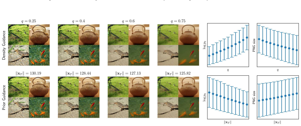
The key object is the generalized instantaneous change-of-variable formula for a continuous normalizing flow, $\frac{d}{dt} \log p_t(x_t) = -\operatorname{div} u_t(x_t) + \nabla \log p_t(x_t)^\top (\tilde u_t(x_t) - u_t(x_t))$, which tracks how the model's marginal density changes when the sample follows a different drift. Density Guidance inverts this formula: instead of computing the density change caused by a new drift, it solves for the drift that produces a desired density change, choosing the solution closest to the original vector field. Score alignment is a secondary device, a tractable condition (checkable even without the score) that predicts when latent rescaling produces monotonic log-density changes.
What would settle it
On a model with a known or very accurately estimated score (e.g., a Gaussian ground-truth diffusion), draw many guided trajectories to a fixed target log-density and measure the achieved empirical log-density of the decoded samples; the central claim is falsified if the achieved values deviate systematically from the target as the target moves away from the median, or if the discrepancy grows with the strength of guidance.
Extended reading notes
Core claim
The central claim is that one can derive an alternative ODE whose trajectories have exactly prescribed log-density evolution: given the score function and the original vector field, the drift $\tilde u_t(x) = u_t(x) + \frac{\operatorname{div} u_t(x) + b_t(x)}{\|\nabla \log p_t(x)\|^2} \nabla \log p_t(x)$ achieves $\frac{d}{dt} \log p_t(x_t) = b_t(x_t)$ while deviating as little as possible from the original flow. With a quantile-based choice of $b_t$, this becomes Density-Guided Sampling, which rescales the score by a factor that depends on the local score norm and the target quantile. The paper further claims that exact log-density control carries over to stochastic sampling by projecting the noise onto the subspace orthogonal to the score and adding a correction term to the drift.
Load-bearing premise
The exact density control holds only if the learned score function and its divergence remain accurate on the guided trajectories, which are deliberately shifted toward less typical regions of the data distribution.
Editorial extensions
If this is right
- Image generation pipelines can set a target quantile of sample log-density, so a user can dial detail continuously from smooth to richly textured without retraining.
- The method inherits the conditional score function, so text-to-image and class-conditional models gain the same detail control by simply replacing the score in the guided drift.
- Stochastic sampling can be used for diversity while the log-density, and hence the detail level, is kept under control, because noise is confined to the subspace orthogonal to the score.
- The score-alignment verification procedure gives model developers a cheap diagnostic for whether latent rescaling will behave monotonically for their model.
Reading between the lines
- The paper's core identity suggests a generic recipe: any flow model with an accurate score estimate can be turned into a likelihood-conditional sampler, which may apply beyond images to scientific generation tasks where marginal likelihood is a meaningful quality signal.
- Because the guided ODE stays closest to the original drift, its trajectories remain near the original model's typical set as long as the score is accurate there; this could make Density Guidance a probe for local score quality, since mismatches between requested and achieved log-density flag regions where the score is unreliable.
- A testable extension would apply the same score-alignment verification to other latent manipulations (e.g., interpolation or principal-component perturbations) to characterize which latent directions reliably control likelihood.
- The quantile-matching choice of $b_t$ depends on the claim that $\sigma_t^2 (\Delta \log p_t + \|\nabla \log p_t\|^2)/\sqrt{2D}$ is approximately standard normal; if that approximation degrades outside high dimension, the implicit quantile mapping would need a different calibrating statistic.
Editorial analysis
A structured set of objections, weighed in public.
Referee Report
Summary. The paper studies how to control the log-density (and thereby the perceived detail) of samples from continuous normalizing flows and diffusion models. It first proposes a score-alignment condition that explains when scaling the latent code (prior guidance) monotonically changes log p0, and shows empirically that the condition holds for most latents in two models. It then derives a modified generative ODE (Density Guidance, Eq. 16) that enforces a prescribed instantaneous log-density change, and extends this to a stochastic sampler (Eq. 25) that injects score-orthogonal noise. The authors claim exact log-density control, demonstrate detail manipulation in Stable Diffusion and EDM2, and provide code.
Significance. If fully supported, the paper would contribute a principled and potentially inexpensive way to control likelihood and image detail in pretrained diffusion models. The score-alignment analysis is a useful explanatory framework, and the derivation of Eq. 16 is algebraically clean. The paper also provides a tractable verification procedure (Eq. 13, Algorithm 1) that does not require knowing intermediate scores. However, the most important claim—exact log-density control—is only valid under idealized conditions that the main experiments do not implement; the practical DGS algorithm is approximate or truncated. The manuscript has the right ingredients but currently overstates what is established.
major comments (4)
- [§4.1, Eq. (19)] Equation (19) contains a logical error. The equality log pt(xt) = log pT(xT) - ∫_T^t bτ dτ = φt(q) can hold only if the initial value satisfies log pT(xT) = φT(q). Since xT is sampled from pT without conditioning on a specific quantile, the choice bt(x) := d/dt φt(q) does not generally drive the sample to the desired quantile. The verification in Appendix E appears to compare the numerically obtained log p0 with the value log pT(xT) - ∫ b_t dt, so it mainly confirms integrator convergence rather than quantile targeting. Please either condition xT on the target quantile, use a feedback controller that drives log pt toward φt(q), or clarify what is actually being verified.
- [§5 and Appendix G] The main image-detail experiments use density guidance only on the interval [T, t*] where log SNR ≥ 1, as stated in Section 4.2; for t < t* the sampler is the unguided PF-ODE. Consequently the final log p0(x0) is not controlled by the chosen quantile q: it equals log pT(xT) - ∫_T^{t*} b_t dt - ∫_{t*}^0 div u_t dt, and the second integral is uncontrolled and starts from a guided, off-typical state. The abstract's claim of "exact log-density control" is therefore not realized by the algorithm used in the main experiments. This is a load-bearing mismatch between the theoretical claim and the empirical setup; it should be stated clearly as an approximation, and ideally the full-trajectory version should be evaluated on the image benchmarks as well.
- [§5 and Appendix G] The stochastic density guidance of Eq. (25) is only approximate. The exact drift in Eq. (120) requires the Rayleigh quotient R(∇^2 log pt, ∇ log pt); the implemented form in Eq. (123) drops this term, justified only by the empirical ratios in Eq. (122). Moreover, the projection P_t makes the diffusion matrix rank-deficient, so the usual Itô corrections must be handled carefully. The manuscript itself uses the word "approximately" in this section, but the abstract claims "precise log-density control" for stochastic sampling. The discrepancy should be reconciled, and the error incurred by omitting the Rayleigh quotient term should be quantified rather than only supported by two empirical measurements.
- [§2.4 and §4] The exactness of Eq. (16) presumes knowledge of the true score and divergence. The experiments rely on neural approximations of these quantities, and the guidance mechanism deliberately moves samples away from the typical set where such approximations are most reliable (as the paper itself notes in Section 4.1). The paper does not provide any diagnostic of how accurate the learned score/divergence are along the guided trajectories. A concrete test—for example, comparing the predicted d log pt/dt against the empirically measured change of log pt along guided trajectories, or measuring the score error on guided vs unguided states—would be needed to support the claim of exact control in practice.
minor comments (5)
- [§5] The text contains a typo: "drfit" should be "drift".
- [References] The reference "Tong, Y., FATRAS, K." should be formatted as "Fatras, K." to match standard capitalization conventions.
- [Appendix E] The text "K3" should presumably be "K = 3", and later the text says K = 128 was used; please clarify the notation and whether the desired log-density is defined per-sample or as a global quantile.
- [Algorithm 1 / Listing 1] In the provided Python code, the branch `if use_omega=False` returns `jnp.dot(v, score_fn(eps, x, key))`, but `eps` is not defined in the function's local scope; as printed, the code would raise a NameError. Please fix the listing.
- [Figure 8] The caption says the distributions of log-likelihoods differ significantly, but it does not state how these log-likelihoods are computed (e.g., via Eq. (3) with a learned score or via an exact method). Please add the computational detail to the caption or text.
Circularity Check
Exact log-density control is a control-law construction; the quantile-matching validation is tautological, though score alignment and DGS experiments provide independent content.
-
self definitional
[Section 4, Eqs. 14-16; abstract claim of 'exact log-density control']
"Suppose that we require an instantaneous density changes over time, constraint: d log pt(xt)/dt = bt(xt) ∈ R (14) for a predetermined bt. To achieve this, we choose a new ODE dxt = ˜utdt, such that its density change from Eq. 4 satisfies bt(xt) = ∇ log pt(xt)T(˜ut(xt) − ut(xt)) − div ut(xt). (15) ... We choose ˜u that is closest to u, which uniquely gives (See Appendix D) ˜ut(x) = ut(x) + div ut(x) + bt(x) ∥∇ log pt(x)∥2 score bias sb(x) ∇ log pt(x). (16)."
Eq. 16 is constructed as the solution of Eq. 15, which is exactly the constraint d log p/dt = b_t. Therefore the guarantee that the guided trajectory's log-density evolves as b_t is true by definition of the drift, not derived from an independent dynamical law. The paper presents this as 'we derive an alternative ODE that guarantees...', but it is control-law synthesis: the exactness is a tautology of the construction. The independent content lies in the later choice of b_t (Eq. 22) and in whether the learned score/divergence stay accurate on the guided, off-typical trajectories.
-
fitted input called prediction
[Appendix E; Section 4.1, Eq. 19]
"We then define bt(x) = d/dt φt, which we estimate with a moving average of finite difference estimates. We found that the difference between the desired values of log-density and the obtained ones goes to zero as we decrease the discretization error (increase the number of sampling steps)."
The desired log-density is φ0(q), the same empirical quantile function whose derivative defines bt. Integrating dφt/dt from t to T reconstructs φT(q)−φt(q) by the fundamental theorem of calculus, so Eq. 19 holds up to an initial offset log pT(xT)−φT(q) and discretization error. The reported >99% correlation therefore measures the numerical integrator's consistency with a definition, not an independent prediction of the method. This is the fitted-input-called-prediction pattern: the target is built from the same quantity used to generate the guidance.
full rationale
The paper contains two genuinely definitional moments. First, the central exactness claim (Eq. 16) is not a derived consequence of an independent law; it is the closed-form solution of the constraint that d log p/dt = b_t (Eq. 15). Thus exact log-density control is guaranteed by construction for any prescribed b_t, and the real content is the choice of b_t and the fidelity of neural score/divergence estimates on guided trajectories. Second, the explicit quantile-matching 'verification' in Appendix E defines b_t from the empirical quantile function φ_t and then compares against the same φ_t; the agreement is an identity up to integration error and an initial offset, not an independent test. These are partial circularities. They do not erase the paper's independent contributions: the score-alignment condition (Section 3) is a mathematical equivalence checked empirically; the DGS score-rescaling form (Eq. 23) and the stochastic projection sampler (Eq. 25) are derived from stated assumptions; and the image-detail experiments are external empirical evidence. The paper's own caveat that guidance is applied only on [T,t*] (Section 4.2) means the exactness theorem is not what the main experiments execute; that is a gap between claim and experiment rather than a circular step. Self-citations to Karczewski et al. (2025) are frequent but not load-bearing here: Eq. 4 is re-derived in Appendix B, and the density/detail correlation is re-examined in Fig. 4. Overall, the derivation chain is mostly self-contained, with two definitional/tautological moments that warrant a moderate circularity score.
Assumptions & free parameters
free parameters (3)
- q (target quantile) =
user-chosen in [0,1]
- t* (guidance threshold) =
log SNR(t*) = 1 (t* ≈ 0.6)
- noise strength φ(t) in stochastic guidance =
φ = r·g(t) for r in {0.1, 0.5, 0.9}; or 0.2g/0.3g in Appendix K
assumptions (4)
- domain assumption The vector field ut and score ∇log pt are known exactly through neural network approximations (Section 2.4).
- standard math The generalized density evolution Eq. 4 (citing Karczewski et al. 2025) is valid for evaluating log pt along a sample following a modified drift ũ.
- ad hoc to paper The empirical asymptotic normality σ_t²(∆log p_t + ||∇log p_t||²)/√(2D) ≈ N(0,1) (Eq. 83) holds for the data distributions used.
- domain assumption Log-density log p0(x0) is a monotone proxy for perceptual detail (from Karczewski et al. 2025 and Fig. 4).
Cite this review
Pith. "Pith review of Devil is in the Details: Density Guidance for Detail-Aware Generation with Flow Models." pith.science (2026). https://pith.science/paper/S2DGCLRO
@misc{pith2026250205807,
  author       = {Pith},
  title        = {Pith review of: Devil is in the Details: Density Guidance for Detail-Aware Generation with Flow Models},
  year         = {2026},
  howpublished = {\url{https://pith.science/paper/S2DGCLRO}},
  note         = {Machine review of arXiv:2502.05807}
}
read the original abstract
Diffusion models have emerged as a powerful class of generative models, capable of producing high-quality images by mapping noise to a data distribution. However, recent findings suggest that image likelihood does not align with perceptual quality: high-likelihood samples tend to be smooth, while lower-likelihood ones are more detailed. Controlling sample density is thus crucial for balancing realism and detail. In this paper, we analyze an existing technique, Prior Guidance, which scales the latent code to influence image detail. We introduce score alignment, a condition that explains why this method works and show that it can be tractably checked for any continuous normalizing flow model. We then propose Density Guidance, a principled modification of the generative ODE that enables exact log-density control during sampling. Finally, we extend Density Guidance to stochastic sampling, ensuring precise log-density control while allowing controlled variation in structure or fine details. Our experiments demonstrate that these techniques provide fine-grained control over image detail without compromising sample quality. Code is available at https://github.com/Aalto-QuML/density-guidance.
Figures


Figures from the paper (19 more)




Reference graph
Works this paper leans on
-
[1]
write newline
" write newline "" before.all 'output.state := FUNCTION n.dashify 't := "" t empty not t #1 #1 substring "-" = t #1 #2 substring "--" = not "--" * t #2 global.max substring 't := t #1 #1 substring "-" = "-" * t #2 global.max substring 't := while if t #1 #1 substring * t #2 global.max substring 't := if while FUNCTION format.date year duplicate empty "emp...
-
[2]
Albergo, M. S. and Vanden-Eijnden, E. Building normalizing flows with stochastic interpolants. In ICLR, 2023
work page 2023
-
[3]
Automatic differentiation in machine learning: A survey
Baydin, A., Pearlmutter, B., Radul, A., and Siskind, J. Automatic differentiation in machine learning: A survey. JMLR, 2018
work page 2018
-
[4]
Neural ordinary differential equations
Chen, R., Rubanova, Y., Bettencourt, J., and Duvenaud, D. Neural ordinary differential equations. In NeurIPS, 2018
work page 2018
-
[5]
A central limit theorem for generalized quadratic forms
de Jong, P. A central limit theorem for generalized quadratic forms. Probability Theory and Related Fields, 75 0 (2): 0 261--277, 1987
work page 1987
-
[6]
On analyzing generative and denoising capabilities of diffusion-based deep generative models
Deja, K., Kuzina, A., Trzcinski, T., and Tomczak, J. On analyzing generative and denoising capabilities of diffusion-based deep generative models. In NeurIPS, 2022
work page 2022
-
[7]
Score-based generative modeling with critically-damped L angevin diffusion
Dockhorn, T., Vahdat, A., and Kreis, K. Score-based generative modeling with critically-damped L angevin diffusion. In ICLR, 2022
work page 2022
-
[8]
A., Welling, M., and van de Meent, J.-W
Eijkelboom, F., Bartosh, G., Naesseth, C. A., Welling, M., and van de Meent, J.-W. Variational flow matching for graph generation. In NeurIPS, 2024
work page 2024
Show all 38 references
-
[9]
Learning normalizing flows from E ntropy- K antorovich potentials
Finlay, C., Gerolin, A., Oberman, A., and Pooladian, A.-A. Learning normalizing flows from E ntropy- K antorovich potentials. arXiv preprint arXiv:2006.06033, 2020
2006 arXiv
-
[10]
T., Bettencourt, J., Sutskever, I., and Duvenaud, D
Grathwohl, W., Chen, R. T., Bettencourt, J., Sutskever, I., and Duvenaud, D. FFJORD : F ree-form continuous dynamics for scalable reversible generative models. In ICLR, 2019
2019
-
[11]
Denoising diffusion probabilistic models
Ho, J., Jain, A., and Abbeel, P. Denoising diffusion probabilistic models. In NeurIPS, 2020
2020
-
[12]
Hutchinson, M. F. A stochastic estimator of the trace of the influence matrix for laplacian smoothing splines. Communications in Statistics-Simulation and Computation, 1989
1989
-
[13]
On a formula concerning stochastic differentials
It \^o , K. On a formula concerning stochastic differentials. Nagoya Mathematical Journal, 3: 0 55--65, 1951
1951
-
[14]
L., Hosseinzadeh, R., Cresswell, J., and Loaiza-Ganem, G
Kamkari, H., Ross, B. L., Hosseinzadeh, R., Cresswell, J., and Loaiza-Ganem, G. A geometric view of data complexity: E fficient local intrinsic dimension estimation with diffusion models. In NeurIPS, 2024
2024
-
[15]
Diffusion models as cartoonists! T he curious case of high density regions
Karczewski, R., Heinonen, M., and Garg, V. Diffusion models as cartoonists! T he curious case of high density regions. In ICLR, 2025
2025
-
[16]
Elucidating the design space of diffusion-based generative models
Karras, T., Aittala, M., Aila, T., and Laine, S. Elucidating the design space of diffusion-based generative models. In NeurIPS, 2022
2022
-
[17]
Guiding a diffusion model with a bad version of itself
Karras, T., Aittala, M., Kynk \"a \"a nniemi, T., Lehtinen, J., Aila, T., and Laine, S. Guiding a diffusion model with a bad version of itself. In NeurIPS, 2024 a
2024
-
[18]
Analyzing and improving the training dynamics of diffusion models
Karras, T., Aittala, M., Lehtinen, J., Hellsten, J., Aila, T., and Laine, S. Analyzing and improving the training dynamics of diffusion models. In CVPR, 2024 b
2024
-
[19]
Variational diffusion models
Kingma, D., Salimans, T., Poole, B., and Ho, J. Variational diffusion models. In NeurIPS, 2021
2021
-
[20]
Flow matching for generative modeling
Lipman, Y., Chen, R., Ben-Hamu, H., Nickel, M., and Le, M. Flow matching for generative modeling. In ICLR, 2023
2023
-
[21]
Flow straight and fast: Learning to generate and transfer data with rectified flow
Liu, X., Gong, C., and Liu, Q. Flow straight and fast: Learning to generate and transfer data with rectified flow. In ICLR, 2023
2023
-
[22]
completely blind
Mittal, A., Soundararajan, R., and Bovik, A. C. Making a “completely blind” image quality analyzer. IEEE Signal processing letters, 2012
2012
-
[23]
W., and Lakshminarayanan, B
Nalisnick, E., Matsukawa, A., Teh, Y. W., and Lakshminarayanan, B. Detecting out-of distribution inputs to deep generative models using typicality. In NeurIPS Bayesian Deep Learning workshop, 2019
2019
-
[24]
High-resolution image synthesis with latent diffusion models
Rombach, R., Blattmann, A., Lorenz, D., Esser, P., and Ommer, B. High-resolution image synthesis with latent diffusion models. In CVPR, 2022
2022
-
[25]
M., Hasan, M
Sami, S. M., Hasan, M. M., Dawson, J., and Nasrabadi, N. Hf-diff: High-frequency perceptual loss and distribution matching for one-step diffusion-based image super-resolution. arXiv, 2024
2024
-
[26]
Generating high fidelity data from low-density regions using diffusion models
Sehwag, V., Hazirbas, C., Gordo, A., Ozgenel, F., and Canton, C. Generating high fidelity data from low-density regions using diffusion models. In CVPR, 2022
2022
-
[27]
The superposition of diffusion models using the it\^o density estimator
Skreta, M., Atanackovic, L., Bose, J., Tong, A., and Neklyudov, K. The superposition of diffusion models using the it\^o density estimator. In ICLR, 2025
2025
-
[28]
Denoising diffusion implicit models
Song, J., Meng, C., and Ermon, S. Denoising diffusion implicit models. In ICLR, 2021 a
2021
-
[29]
P., Kumar, A., Ermon, S., and Poole, B
Song, Y., Sohl-Dickstein, J., Kingma, D. P., Kumar, A., Ermon, S., and Poole, B. Score-based generative modeling through stochastic differential equations. In ICLR, 2021 b
2021
-
[30]
Consistency models
Song, Y., Dhariwal, P., Chen, M., and Sutskever, I. Consistency models. In ICML, 2023
2023
-
[31]
Improving and generalizing flow-based generative models with minibatch optimal transport
Tong, A., FATRAS, K., Malkin, N., Huguet, G., Zhang, Y., Rector-Brooks, J., Wolf, G., and Bengio, Y. Improving and generalizing flow-based generative models with minibatch optimal transport. TMLR, 2024
2024
-
[32]
Score-based generative modeling in latent space
Vahdat, A., Kreis, K., and Kautz, J. Score-based generative modeling in latent space. In NeurIPS, 2021
2021
-
[33]
and Vastola, J
Wang, B. and Vastola, J. Diffusion models generate images like painters: an analytical theory of outline first, details later. arXiv preprint arXiv:2303.02490, 2023
2023 arXiv
-
[34]
C., Sheikh, H
Wang, Z., Bovik, A. C., Sheikh, H. R., and Simoncelli, E. P. Image quality assessment: from error visibility to structural similarity. IEEE transactions on image processing, 2004
2004
-
[35]
Normalizing flow neural networks by JKO scheme
Xu, C., Cheng, X., and Xie, Y. Normalizing flow neural networks by JKO scheme. In NeurIPS, 2024
2024
-
[36]
Scalable stochastic gradient R iemannian L angevin dynamics in non-diagonal metrics
Yu, H., Hartmann, M., Williams, B., and Klami, A. Scalable stochastic gradient R iemannian L angevin dynamics in non-diagonal metrics. TMLR, 2023
2023
-
[37]
A., Shechtman, E., and Wang, O
Zhang, R., Isola, P., Efros, A. A., Shechtman, E., and Wang, O. The unreasonable effectiveness of deep features as a perceptual metric. In CVPR, 2018
2018
-
[38]
V., and Ramos, F
Zhi, W., Lai, T., Ott, L., Bonilla, E. V., and Ramos, F. Learning ODE s via diffeomorphisms for fast and robust integration. In ICML, 2022
2022
Reviewed August 8, 2026 · model on record in the stance chip above.
Discussion (0). Continue with ORCID to comment.