REVIEW 3 major objections 5 minor 38 references
Deep Ritz method with Fourier feature mapping: A deep learning approach for solving variational models of microstructure
T0 review · 3 major / 5 minor · reviewed 2026-08-08 · deepseek-v4-flash
Pith's one-line read Fourier features give Deep Ritz fine-scale solutions without deeper networks.
desk verdict Fourier features help DRM produce more high-frequency structure on non-convex benchmarks, but missing energy values for the no-minimizer problems leave the 'solving' claim only partially supported. read the letter →
The pith
A machine-rendered reading of the paper's core claim, the machinery that carries it, and where it could break.
The reading
What carries the argument
The load-bearing object is the DRM neural tangent kernel, the matrix-valued kernel $K(x_m,x_n;\theta)=\nabla_\theta U_m(\theta)[\nabla_\theta U_n(\theta)]^T$, where $U_n=(u(x_n),u'(x_n))^T$ stacks the network output and its spatial derivative. This kernel enters a Gram matrix $M_X$ whose spectral decomposition $D_X M_X = Q\Lambda Q^T$ sets the per-direction convergence rates in Theorem 1. The second ingredient is the Fourier feature map; by sending the input to the unit circle $S^1$ (or adjoining $x$ in 2D), it makes the NTK eigenvalue decay quadratic in the eigen-index, which is what allows the method to learn high frequencies.
What would settle it
Compute $I(u)$ for the DRM&FM outputs of problems (17) and (18) and test whether it approaches zero as Fourier frequency or training epochs increase; if the energy stays bounded away from zero, the visible oscillations are not minimizing sequences.
Extended reading notes
Core claim
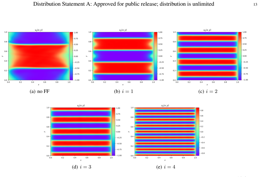
On its own terms, the central claim is that DRM inherits the spectral-bias pathology of neural networks: the gradient-descent dynamics of the loss decompose into eigen-directions of a DRM-specific NTK, and directions with small eigenvalues converge exponentially slowly. Theorem 1 states that under lazy training, convexity of the Lagrangian in $(u,u')$, and positive definiteness of the Gram matrix, the component of the gradient along eigen-direction $q_i$ decays as $e^{-\eta \lambda_i t/|X|}$. Fourier feature mapping $\delta(x) = (\sin(2^i \pi x), \cos(2^i \pi x))$ in 1D (and $(x, \sin(2^i \pi x), \cos(2^i \pi x))$ in 2D) maps the input onto a submanifold on which the NTK eigenspectrum has quadratic decay, which the paper takes to homogenize learning across scales. The numerical section demonstrates that with this mapping, deeper networks are not needed: the number of transitions between preferred states (and twin bands in 2D) grows with the Fourier frequency, and a regularization term controls smoothness and interface spacing.
Load-bearing premise
The load-bearing premise is that a network output whose plot shows many transitions between preferred states is a minimizing sequence; for the benchmarks with no true minimizer the paper does not report the energy values that would show approach to the infimum.
Editorial extensions
If this is right
- For the 1D double-well problem (15), plain DRM with 5, 7, and 9 hidden layers produces only one transition between the two preferred slopes, while DRM&FM with Fourier frequencies $4\pi$ and $8\pi$ produces 4 and 8 transitions at the same depth.
- For the non-attaining 1D benchmark (17), DRM&FM at frequency $2\pi$ produces about 12 transitions with a fixed 3-hidden-layer network, rivaling a 7-hidden-layer plain DRM; higher Fourier frequencies increase the transition count.
- For the 2D twin-branching problem (18), Fourier frequencies $2\pi,4\pi,8\pi,16\pi$ produce 4, 8, 15, and 32 twin bands, whereas plain DRM with 7 hidden layers stalls at an unstable state.
- Adding the regularization term $\varepsilon^2 u_{yy}^2$ smooths the minimizing sequences and limits the number of interfaces; larger $\varepsilon$ yields lower-frequency solutions.
- The NTK analysis identifies the eigenvalue spectrum of the DRM kernel as the mechanism behind spectral bias, so Fourier features target the convergence-rate bottleneck directly rather than relying on network depth.
Reading between the lines
- A testable extension is to report the energy $I(u)$ of the outputs for benchmarks (17) and (18) and check whether it approaches the infimum; the paper's evidence is transition counts in plots, so an energy-based check would directly settle whether the outputs are minimizing sequences.
- The observed tie between Fourier frequency and transition count suggests an adaptive frequency schedule, where the input-map frequencies are annealed or selected from the current energy landscape instead of fixed at $i=1,\dots,4$.
- If the quadratic-decay NTK result extends beyond the 1D $W=W(x,u)$ case, the same input mapping may transfer to other non-convex variational problems with oscillatory minimizers, such as micromagnetics or phase-field models.
- The paper leaves the non-convex version of Theorem 1 open; a rigorous treatment would need to replace the convexity and lazy-training assumptions with a variational analysis of the non-convex landscape, which the conclusions identify as future work.
Editorial analysis
A structured set of objections, weighed in public.
Referee Report
Summary. The paper proposes combining the Deep Ritz Method (DRM) with Fourier feature mapping (DRM&FM) to solve non-convex variational problems arising in microstructure modeling. The authors first present a neural tangent kernel (NTK) analysis for DRM, arguing that DRM suffers from spectral bias because convergence along different directions is controlled by the eigenvalues of the NTK Gram matrix. They then argue that Fourier feature mapping, by mapping inputs onto the unit circle, can lead to a quadratically decaying NTK spectrum, which may alleviate spectral bias. Numerically, the paper studies three benchmarks: a 1D double-well problem (15) with attained minimizers, a 1D double-well problem with a lower-order term (17) whose infimum is zero but is not attained, and a 2D twin-branching problem (18) also without an attained minimizer. For each problem, the authors show derivative plots and count transitions between preferred states, comparing DRM with and without Fourier features at various network depths and frequencies. The central claim is that DRM&FM generates high-frequency, multiscale minimizing sequences independently of network depth, while plain DRM does not.
Significance. If the central claim is validated, the paper offers a practical, mesh-free alternative to finite elements for a difficult class of non-convex, microstructure-scale variational problems, and it provides a useful NTK-based heuristic for why Fourier features help DRM. The concrete NTK derivation for DRM in Section 3.1, with the explicit loss dynamics (14) and the spectral decomposition in Theorem 1, is a valuable contribution in itself, even though its assumptions are not met by the benchmarks. The numerical experiments cover both 1D and 2D settings and include a regularization study in Section 4.4, which strengthens the empirical picture. However, the evidence supporting the main 'solving' claim is incomplete because no energy values are reported for the no-minimizer benchmarks, and the depth-independence claim is qualified by a counterexample in Figure 4(c). The paper is therefore of interest to the community, but its central numerical claim requires additional verification before it can be accepted as stated.
major comments (3)
- [Sections 4.2 and 4.3, Eqs. (17) and (18)] The central claim that DRM&FM produces minimizing sequences for the no-minimizer benchmarks is not supported by the reported evidence. For problems (17) and (18), the infimum is zero but is not attained, so a function with many transitions can still have energy arbitrarily far from the infimum if its derivative wanders away from the wells or if the lower-order term (for (17)) contributes significantly. The paper reports only transition counts and derivative plots (Figures 5-10) without ever reporting the computed energy I(û) at any epoch or at convergence. I strongly recommend adding energy trajectories or final energy values, and ideally a comparison with the known infimum, for all benchmarks and for both DRM and DRM&FM at the frequencies and depths tested. Without this, the assertion that DRM&FM 'generates minimizing sequences' is not quantitatively supported.
- [Figure 4(c) and Section 4.1] The abstract and Sections 1 and 4 claim that Fourier feature mapping enables high-frequency solutions 'independently of the depth of the DNN' or 'independently of the depth' (Section 1). Figure 4(c) directly contradicts this for benchmark (15): with Fourier frequency i=4, the 5- and 7-layer networks produce 32 transitions, but the 9-layer network produces 16 transitions. The text in Section 4.1 also states that 'one cannot quantify the relationship between mapping frequency and number of transitions within the domain,' and Section 4.2 admits the frequency-transition relationship was not investigated. The depth-independence claim should either be restricted to the frequencies and depths where it actually holds, or the authors should provide a more systematic study that quantifies the dependence on depth, frequency, and training epochs. As written, the claim is too strong relative to the presented evidence.
- [Section 3.1, Theorem 1] Theorem 1 requires W to be strictly convex in (u, u') and the Hessian blocks D_X to be positive definite, as stated in the theorem assumptions. The benchmarks studied in Section 4 are all non-convex, and the authors themselves note in the remark following Theorem 1 that 'for a non-convex Lagrangian W, the convergence of ∇U ¯W_X requires a more refined analysis.' This means the NTK-based spectral-bias explanation is rigorously valid only for a different class of problems than the ones actually solved. The paper should be explicit that Theorem 1 is a heuristic motivation, not a proof of the observed behavior for the non-convex benchmarks. Alternatively, the authors could include a finite-width or direct eigenvalue analysis for the specific non-convex W used in the experiments, or at least empirically examine the decay of the NTK eigenvalues for those W.
minor comments (5)
- [Section 2] The optimizer is referred to as 'Adams Optimizer' in Sections 4.1, 4.2, and 4.3; the standard name is 'Adam' (Kingma and Ba, reference [26]). Please correct this typo throughout.
- [Figure 5 caption] The caption of Figure 5 says 'First Row (a)-(c): DRM approximation to (17) with ReLU activation function, ε = 0, η = 1.0 × 10⁻⁴' and 'Second Row (d)-(f)', but the notation 'ε = 0' is unexplained in the 1D context; the epsilon parameter is defined only for the 2D regularized problem (19). Please clarify what ε refers to in Figures 5 and 6.
- [Section 4.1, Figure 4 caption] The caption of Figure 4 states that the Fourier mapping is 'of frequency δ(x) = (sin(2iπx), cos(2iπx))' but the frequency is 2iπ, not i; the text in Section 4.1 says 'a Fourier mapping of frequency 4π' for i=2, which is consistent. Please make the caption consistent with the text to avoid confusion.
- [Appendix B] Appendix B states that the eigenvalues of the Gram matrix M_X are approximately λ_k ≈ nΛ_k for large n, and the main text in Section 3.2 uses the 'quadratic decay' of the NTK eigenvalues from reference [23]. However, the connection between the decay rate of the integral operator eigenvalues and the decay rate of the Gram matrix eigenvalues for finite n is only sketched. A brief comment on the finite-n regime would help the reader gauge how directly the O(k^{-2}) result applies to the numerical experiments with n = 128 or n = 1000.
- [Section 5, conclusions] The concluding sentence acknowledges that the method 'lacks a theoretical foundation to quantify solution accuracy for the considered minimization problems.' This is honest and appropriate, but given that the benchmarks are exactly of that type, the paper should also present empirical energy values as the substitute form of accuracy verification, which is currently missing (see major comment 1).
Circularity Check
No significant circularity: the Fourier features are chosen a priori, the NTK analysis cites external results, and the reported transition counts are evaluation metrics rather than fitted targets.
full rationale
The paper's claimed derivation chain is: (i) DRM minimizes the energy functional via SGD; (ii) Theorem 1 and the NTK computation show that the linearized loss dynamics converge along eigen-directions with rates governed by eigenvalues of the NTK Gram matrix; (iii) Section 3.2 argues that a Fourier feature input map delta(x) = [sin x, cos x] makes the relevant kernel's eigenvalue spectrum decay quadratically, citing Geifman et al. and Chen & Xu as external sources; (iv) Section 4 reports transition counts for the three benchmarks with and without Fourier features. I find no step in which a target output is defined in terms of the method's own fitted parameters, nor any load-bearing self-citation: the baseline [21] and the NTK eigenvalue results [23,24] are not by the present authors, and the Fourier frequencies are chosen before training rather than fit to the reported transition counts. The success metric (number of transitions between preferred states) is not used as a training signal, and the paper explicitly notes that 'the authors did not investigate the relationship between the frequency of the Fourier mapping and the number of transitions within the solution for this 1D problem,' so the observed correlation does not reduce to a fitted identity. The admitted lack of a theoretical accuracy bound in Section 5 ('its nonlinear nature lacks a theoretical foundation to quantify solution accuracy for the considered minimization problems') and the inconsistent 9-layer result in Fig. 4(c) are genuine evidentiary limitations for the 'solving' and 'depth independence' claims, but they are support gaps, not circular reductions. Since no specific circular step can be quoted from the paper, the appropriate finding is no significant circularity.
Assumptions & free parameters
free parameters (4)
- Fourier feature frequency i =
2, 4, 8, 16 (cycle frequencies 2iπ)
- Boundary penalty λ =
500
- Activation smoothing ρ =
0.1
- Training epochs =
100,000 to 500,000 depending on experiment
assumptions (3)
- domain assumption Lazy training / NTK linearization
- ad hoc to paper Strict convexity of W in (u,u')
- domain assumption Quadratic NTK eigenvalue decay on S^1 transfers to the actual Fourier features
Cite this review
Pith. "Pith review of Deep Ritz method with Fourier feature mapping: A deep learning approach for solving variational models of microstructure." pith.science (2026). https://pith.science/paper/5GE4AFBY
@misc{pith2026250206865,
  author       = {Pith},
  title        = {Pith review of: Deep Ritz method with Fourier feature mapping: A deep learning approach for solving variational models of microstructure},
  year         = {2026},
  howpublished = {\url{https://pith.science/paper/5GE4AFBY}},
  note         = {Machine review of arXiv:2502.06865}
}
read the original abstract
This paper presents a novel approach that combines the Deep Ritz Method (DRM) with Fourier feature mapping to solve minimization problems comprised of multi-well, non-convex energy potentials. These problems present computational challenges as they lack a global minimum. Through an investigation of three benchmark problems in both 1D and 2D, we observe that DRM suffers from spectral bias pathology, limiting its ability to learn solutions with high frequencies. To overcome this limitation, we modify the method by introducing Fourier feature mapping. This modification involves applying a Fourier mapping to the input layer before it passes through the hidden and output layers. Our results demonstrate that Fourier feature mapping enables DRM to generate high-frequency, multiscale solutions for the benchmark problems in both 1D and 2D, offering a promising advancement in tackling complex non-convex energy minimization problems.
Figures


Figures from the paper (7 more)


Reference graph
Works this paper leans on
-
[1]
K. Bhattacharya, Microstructure of martensite: why it forms and how it gives rise to the shape-memory effect, V ol. 2, Oxford University Press, 2003
work page 2003
-
[2]
Dacorogna, Direct methods in the calculus of variations, V ol
B. Dacorogna, Direct methods in the calculus of variations, V ol. 78, Springer Science & Business Media, 2007
work page 2007
-
[3]
Luskin, On the computation of crystalline microstructure, Acta numerica 5 (1996) 191–257
M. Luskin, On the computation of crystalline microstructure, Acta numerica 5 (1996) 191–257
work page 1996
-
[4]
C. Carstensen, Ten remarks on nonconvex minimisation for phase transition simulations, Computer Methods in Applied Mechanics and Engineering 194 (2) (2005) 169–193
work page 2005
-
[5]
M. K. Gobbert, A. Prohl, A discontinuous finite element method for solving a multiwell problem, SIAM journal on numerical analysis 37 (1) (1999) 246–268
work page 1999
-
[6]
C. Carstensen, Numerical analysis of microstructure, Theory and Numerics of Differential Equations: Durham 2000 (2001) 59–126
work page 2001
-
[7]
S. Bartels, C. Carstensen, K. Hackl, U. Hoppe, Effective relaxation for microstructure simulations: algorithms and applications, Computer Methods in Applied Mechanics and Engineering 193 (48-51) (2004) 5143–5175
work page 2004
-
[8]
C. Carstensen, P. Plecháˇc, Numerical solution of the scalar double-well problem allowing microstructure, Mathe- matics of Computation 66 (219) (1997) 997–1026
work page 1997
Show all 38 references
-
[9]
R. A. Nicolaides, N. J. Walkington, Computation of microstructure utilizing young measure representations, Journal of intelligent material systems and structures 4 (4) (1993) 457–462
1993
-
[10]
Aranda, P
E. Aranda, P. Pedregal, Numerical approximation of non-homogeneous, non-convex vector variational problems, Numerische Mathematik 89 (2001) 425–444
2001
-
[11]
Carstensen, T
C. Carstensen, T. Roubíˇcek, Numerical approximation of young measuresin non-convex variational problems, Numerische Mathematik 84 (2000) 395–415
2000
-
[12]
Hornik, M
K. Hornik, M. Stinchcombe, H. White, Universal approximation of an unknown mapping and its derivatives using multilayer feedforward networks, Neural networks 3 (5) (1990) 551–560
1990
-
[13]
Hornik, Approximation capabilities of multilayer feedforward networks, Neural networks 4 (2) (1991) 251–257
K. Hornik, Approximation capabilities of multilayer feedforward networks, Neural networks 4 (2) (1991) 251–257
1991
-
[14]
Raissi, P
M. Raissi, P. Perdikaris, G. E. Karniadakis, Physics-informed neural networks: A deep learning framework for solving forward and inverse problems involving nonlinear partial differential equations, Journal of Computational physics 378 (2019) 686–707. Distribution Statement A: ...
2019
-
[15]
Sirignano, K
J. Sirignano, K. Spiliopoulos, Dgm: A deep learning algorithm for solving partial differential equations, Journal of computational physics 375 (2018) 1339–1364
2018
-
[16]
Yu, et al., The deep ritz method: a deep learning-based numerical algorithm for solving variational problems, Communications in Mathematics and Statistics 6 (1) (2018) 1–12
B. Yu, et al., The deep ritz method: a deep learning-based numerical algorithm for solving variational problems, Communications in Mathematics and Statistics 6 (1) (2018) 1–12
2018
-
[17]
J. Han, A. Jentzen, et al., Deep learning-based numerical methods for high-dimensional parabolic partial differential equations and backward stochastic differential equations, Communications in mathematics and statistics 5 (4) (2017) 349–380
2017
-
[18]
Grohs, F
P. Grohs, F. Hornung, A. Jentzen, P. V on Wurstemberger, A proof that artificial neural networks overcome the curse of dimensionality in the numerical approximation of black-scholes partial differential equations, arXiv preprint arXiv:1809.02362 (2018)
2018 arXiv
-
[19]
Rahaman, A
N. Rahaman, A. Baratin, D. Arpit, F. Draxler, M. Lin, F. Hamprecht, Y . Bengio, A. Courville, On the spectral bias of neural networks, in: International Conference on Machine Learning, PMLR, 2019, pp. 5301–5310
2019
-
[20]
S. Wang, H. Wang, P. Perdikaris, On the eigenvector bias of fourier feature networks: From regression to solving multi-scale pdes with physics-informed neural networks, Computer Methods in Applied Mechanics and Engineering 384 (2021) 113938
2021
-
[21]
X. Chen, P. Rosakis, Z. Wu, Z. Zhang, Solving nonconvex energy minimization problems in martensitic phase transitions with a mesh-free deep learning approach, Computer Methods in Applied Mechanics and Engineering 416 (2023) 116384
2023
-
[22]
Tancik, P
M. Tancik, P. P. Srinivasan, B. Mildenhall, S. Fridovich-Keil, N. Raghavan, U. Singhal, R. Ramamoorthi, J. T. Barron, R. Ng, Fourier features let networks learn high frequency functions in low dimensional domains, NeurIPS (2020)
2020
-
[23]
Geifman, A
A. Geifman, A. Yadav, Y . Kasten, M. Galun, D. Jacobs, B. Ronen, On the similarity between the laplace and neural tangent kernels, Advances in Neural Information Processing Systems 33 (2020) 1451–1461
2020
-
[24]
L. Chen, S. Xu, Deep neural tangent kernel and laplace kernel have the same rkhs, arXiv preprint arXiv:2009.10683 (2020)
2020 arXiv
-
[25]
Weinan, B
E. Weinan, B. Yu, The deep ritz method: A deep learning-based numerical algorithm for solving variational problems, Communications in Mathematics and Statistics 6 (1) (2018) 1–12
2018
-
[26]
D. P. Kingma, J. Ba, Adam: A method for stochastic optimization, arXiv preprint arXiv:1412.6980 (2014)
2014 arXiv
-
[27]
Jacot, F
A. Jacot, F. Gabriel, C. Hongler, Neural tangent kernel: Convergence and generalization in neural networks, Advances in neural information processing systems 31 (2018)
2018
-
[28]
S. S. Du, X. Zhai, B. Poczos, A. Singh, Gradient descent provably optimizes over-parameterized neural networks, arXiv preprint arXiv:1810.02054 (2018)
2018 arXiv
-
[29]
Chizat, E
L. Chizat, E. Oyallon, F. Bach, On lazy training in differentiable programming, Advances in neural information processing systems 32 (2019)
2019
-
[30]
J. Lee, L. Xiao, S. Schoenholz, Y . Bahri, R. Novak, J. Sohl-Dickstein, J. Pennington, Wide neural networks of any depth evolve as linear models under gradient descent, Advances in neural information processing systems 32 (2019)
2019
-
[31]
Arora, S
S. Arora, S. S. Du, W. Hu, Z. Li, R. R. Salakhutdinov, R. Wang, On exact computation with an infinitely wide neural net, Advances in neural information processing systems 32 (2019)
2019
-
[32]
Rahimi, B
A. Rahimi, B. Recht, Random features for large-scale kernel machines, Advances in neural information processing systems 20 (2007)
2007
-
[33]
Muller, Singular perturbations as a selection criterion for periodic minimizing sequences, Calc
S. Muller, Singular perturbations as a selection criterion for periodic minimizing sequences, Calc. Var. Partial Differential Equations 1 (2) (1993) 169–204
1993
-
[34]
R. V . Kohn, F. Otto, Small surface energy, coarse-graining, and selection of microstructure, Physica D: Nonlinear Phenomena 107 (2) (1997) 272–289
1997
-
[35]
Müller, Variational models for microstructure and phase transitions, Lecture Notes in Math
S. Müller, Variational models for microstructure and phase transitions, Lecture Notes in Math. 1713 (1999) 85–210
1999
-
[36]
R. V . Kohn, S. Müller, Relaxation and regularization of nonconvex variational problems, Rendiconti del Seminario Matematico e Fisico di Milano 62 (1) (1992) 89–113
1992
-
[37]
Dondl, B
P. Dondl, B. Heeren, M. Rumpf, Optimization of the branching pattern in coherent phase transitions, Comptes Rendus Mathematique 354 (6) (2016) 639–644. Distribution Statement A: Approved for public release; distribution is unlimited 17
2016
-
[38]
C. K. Williams, C. E. Rasmussen, Gaussian processes for machine learning, V ol. 2, MIT press Cambridge, MA, 2006
2006
Reviewed August 8, 2026 · model on record in the stance chip above.
Discussion (0). Continue with ORCID to comment.