REVIEW 5 major objections 5 minor 50 references
An Alternative Approach to the Exact Solution of FRW-Type Spacetime with a Generalized Chaplygin Gas
T0 review · 5 major / 5 minor · reviewed 2026-08-08 · deepseek-v4-flash
Pith's one-line read The paper claims that a first-order binomial truncation of the Friedmann equation for a generalized Chaplygin gas is exactly solved by a(t)=a0 sinh^n(ωt), and that this solution supplies the missing transition from deceleration to…
desk verdict The alternative solution doesn't solve the equation it's derived from unless c=B, and the paper's own fit rules that out; the rest is routine GCG cosmology with a circular H(z) comparison. read the letter →
The pith
A machine-rendered reading of the paper's core claim, the machinery that carries it, and where it could break.
The reading
What carries the argument
The load-bearing object is the first-order binomial truncation of the Friedmann equation, eq (36): the right-hand side [B + c $a^{{-3(1+α)}}$]^{1/(1+α)} is replaced by $B^{{1/(1+α)}}$ + [c/((1+α)$B^{{α/(1+α)}}$)] $a^{{-3(1+α)}}$. The proposed solution a(t)=a0 $\sinh$^n(ωt) with a0=(1/(1+α))^{1/[3(1+α)]}, n=2/[3(1+α)], and ω=(√3/2)(1+α)$B^{{1/[2(1+α)]}}$ makes the left-hand side $3H^{2}$ a sum of a constant and a $coth^{2}$(ωt) term, and the paper uses this identity to evaluate density, pressure, deceleration, flip time, effective equation of state, and jerk.
What would settle it
Substitute the proposed scale factor a(t)=a0 $\sinh$^n(ωt) into eq (36) using the paper's own best-fit values (Ωm=0.248, Bs=0.7532, α=0.0051) and compare the coefficients of $a^{{-3(1+α)}}$ on both sides: the equation demands c/[(1+α)$B^{{α/(1+α)}}$] while the proposed solution supplies $B^{{1/(1+α)}}$/(1+α), and these are equal only if c=B, which the fit contradicts. A reader can perform this substitution and see the equality fail at the fitted parameters.
Extended reading notes
Core claim
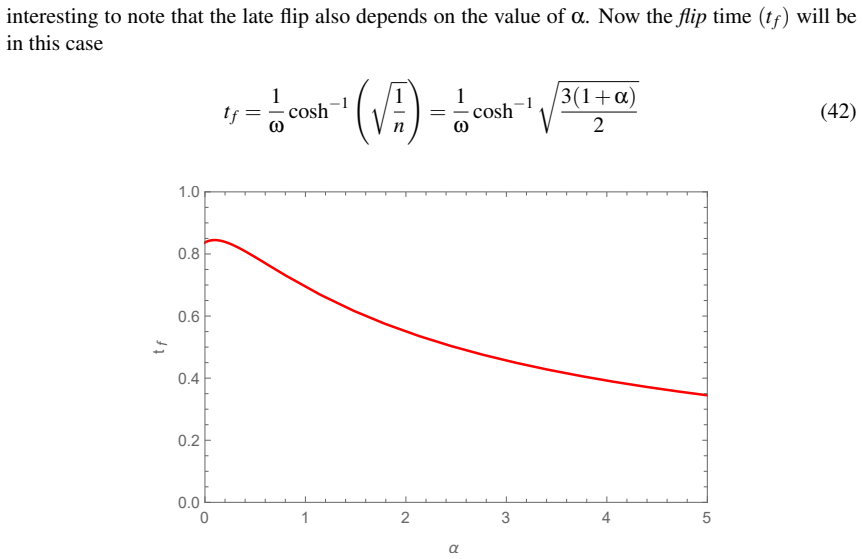
On the paper's own terms, the central discovery is that the first-order approximated Friedmann equation (36) has an exact solution of the form a(t)=a0 $\sinh$^n(ωt), where the constants are fixed uniquely by α and B. From that single formula the paper obtains the energy density and pressure as $coth^{2}$(ωt) expressions, an effective equation of state that runs from 0 to −1, a deceleration parameter that flips from positive to negative at t_f=(1/ω)$\cosh$^{-1}(√(3(1+α)/2)), and a jerk parameter that settles to 1. The paper further checks the flip condition through the Raychaudhuri equation and finds the same flip time and flip redshift. In the paper's interpretation, this closes the gap between the two extremal regimes of the generalized Chaplygin gas and gives a ΛCDM-like late-time attractor without an explicit cosmological constant.
Load-bearing premise
The derivation of the exact sinh solution silently requires c=B, that is, the integration constant of the density integral must equal the Chaplygin parameter B; without that equality, eq (37) does not satisfy the truncated Friedmann equation (36), and the paper does not state or justify this condition.
Editorial extensions
If this is right
- The GCG universe described by eq (37) has an explicit flip time t_f=(1/ω)cosh^{-1}(√(3(1+α)/2)), and smaller α pushes the flip to later times.
- At large cosmic time the solution reaches q=-1, w_eff=-1, and j=1, so it reproduces ΛCDM expansion without a cosmological constant.
- The fitted Hubble-57 parameters give a present age around 13.5 Gyr and a redshift at flip z_f>0, satisfying the requirement that the universe is accelerating today.
- The Raychaudhuri equation reproduces the same flip time and flip redshift, which the paper takes as evidence that the acceleration flip is a robust feature of the solution.
Reading between the lines
- Beyond the paper's claims: direct substitution shows that eq (37) solves eq (36) only when the integration constant c equals the Chaplygin parameter B; the paper never states this condition, and its best-fit values (Ωm≈0.248, Bs≈0.7532, α≈0.0051) give c/B≈0.33, so for the fitted model the proposed scale factor does not satisfy the truncated equation.
- Solving the truncated equation without the c=B shortcut would introduce c/B as an extra parameter, and the resulting correction to the scale factor and flip time is a natural next calculation.
- The same first-order sinh construction applies to any fluid whose Friedmann right-hand side is a two-term binomial in a^{-3(1+α)}, so the method generalizes to other unified dark-sector models.
- Comparing eq (37) with a numerical integration of the full equation (11) at the fitted parameters would quantify how much accuracy is lost by dropping the higher-order terms.
Editorial analysis
A structured set of objections, weighed in public.
Referee Report
Summary. The paper studies the generalized Chaplygin gas (GCG) as the matter content of a flat FRW universe, with equation of state p = -B/ρ^α. After deriving the density as ρ = [B + c a^{-3(1+α)}]^{1/(1+α)} and the Friedmann equation (11), the author proposes a first-order binomial approximation, Eq. (36), and claims the exact solution a(t) = a0 sinh^n(ωt) with n = 2/[3(1+α)], ω = (√3/2)(1+α) B^{1/[2(1+α)]}, a0 = [1/(1+α)]^{1/[3(1+α)]}. On this basis the paper derives expressions for the density, pressure, effective equation of state, deceleration parameter, flip time, flip redshift, and jerk parameter, and then fits the model to the Hubble-57 dataset using both Ω_m- and B_s-parametrizations. The same framework is re-examined with the Raychaudhuri equation. The central claim is that the alternative approach supplies an explicit analytic late-time dynamics for the GCG that reproduces early deceleration and late acceleration and is consistent with observations.
Significance. If the claimed exact solution and its derived cosmological consequences were correct, the paper would provide a useful explicit analytic approximation for the late-time evolution of the GCG model, including a closed-form flip time. The paper also compiles a large Hubble-57 dataset and attempts parameter constraints in two parameterizations. However, the central derivation is not sound: the proposed solution satisfies the approximate Friedmann equation only under a hidden condition on the integration constant c, and several of the derived formulas contain algebraic errors. The observational comparison is partly tautological because the same fitted equation is used to generate both curves. These issues are load-bearing: the 'exact solution' framing, the flip-time results, and the alternative-approach fits rest on incorrect algebra. The paper does not ship reproducible code or machine-checked derivations. Overall, despite a worthwhile ambition, the manuscript in its current form does not establish its main claims.
major comments (5)
- [§4, Eqs. (36)–(37)] The proposed solution does not solve Eq. (36) for general c, and the required condition is never stated. Substituting a(t) = a0 sinh^n(ωt) gives H = nω coth(ωt) and, with the stated n, ω, a0, one obtains 3H^2 = B^{1/(1+α)} [1 + (1/(1+α)) a^{-3(1+α)}]. Eq. (36) instead has the coefficient c/[(1+α)B^{α/(1+α)}] multiplying a^{-3(1+α)}. Equality holds only when c = B. This condition is absent from the paper and is contradicted by its own fits: with Ω_m = 0.248 and B_s = 0.7532 from Tables 4 and 6, one has c/B = Ω_m / B_s^{1+α} ≈ 0.33, not 1. Consequently Eqs. (38)–(46) and all quantities derived from Eq. (37), including the flip time and the alternative-approach H(z) fits, are not supported for the fitted model.
- [§4, Eqs. (38)–(40)] The density and pressure expressions are not consistent with the solution (37). From Eq. (37), the exact density is ρ = 3H^2 = B^{1/(1+α)}[1 + (1/(1+α)) a^{-3(1+α)}], not Eq. (38), which omits the 1/(1+α) factor. Equation (40) also contains algebraic errors: from (38)–(39) one would get w_e = -(1 - α(1+z)^{3(1+α)})/(1 + (1+z)^{3(1+α)}), which tends to α as z→∞, contradicting the text's claim that w_e → -1 in the late universe. The first expression in Eq. (40) is also not equivalent to the second; direct algebra from (37) gives w_e = α - (1+α) tanh^2(ωt), with a different asymptotic behavior. Thus Eqs. (38)–(40) are internally inconsistent and cannot be used as the basis for the Raychaudhuri analysis in Section 5, Case 2.
- [§4, Eqs. (41)–(43)] Equation (41) drops a factor of (1+α) in the redshift variable. From Eq. (37), cosh^2(ωt) = 1 + (1+α)(1+z)^{3(1+α)} and 2/n = 3(1+α), so the correct expression is q = 1/[n(1+(1+α)(1+z)^{-2/n})] - 1, not q = 1/[n(1+(1+z)^{-2/n})] - 1. The error propagates to the flip redshift: the correct solution of q=0 is z_f = [n(1+α)/(1-n)]^{n/2} - 1, not Eq. (43). Since this flip redshift is used to derive the constraint α < 1/3, the constraint is based on an incorrect formula.
- [§4, Eqs. (45)–(46)] Equation (45) is not normalized to H0 at z=0 and does not match the first-order expansion of the exact Friedmann equation. Direct substitution of z=0 into Eq. (45) does not give H = H0 unless a special relation holds among Ω_m, α, and the prefactor. The correct first-order expansion of Eq. (11) is H = H0 (1-Ω_m)^{1/[2(1+α)]} [1 + (1/(1+α)) (Ω_m/(1-Ω_m)) (1+z)^{3(1+α)}]^{1/2}, which differs from Eq. (45) in both the prefactor and the coefficient of (1+z)^{3(1+α)}. Equation (46) is also not a consequence of the solution (37); for c = B, the relation B_s = (1+α)/(2+α) would follow, giving B_s ≈ 0.501 for α ≈ 0.005, far from the fitted B_s = 0.7532. The alternative-approach parameter constraints therefore cannot be considered valid.
- [§3.4, Fig. 5] The comparison in Fig. 5(b) is tautological. The 'best-fit graph' is obtained by fitting the model H(z) of Eq. (32) to the Hubble-57 data, and the 'theoretical graph' is the same Eq. (32) evaluated at the same best-fit parameters. The two curves therefore coincide by construction, and the agreement carries no independent confirmation of the model. A meaningful test would compare the fitted model to a non-parametric reconstruction from the data or to a dataset not used in the fit. The corresponding claims in the abstract and in Section 7 ('excellent agreement with observational data') should be calibrated accordingly.
minor comments (5)
- [§3.4, Eq. (33)] The χ^2 sum in Eq. (33) is written with an upper limit of 30, although the paper states that the Hubble-57 dataset contains 57 data points; the sum should run over all 57 points (or the text should explain the truncated range).
- [Table 1] The error entries in Table 1 use '∓' where '±' is meant; the sign conventions are inconsistent.
- [§4, after Eq. (36)] The justification for the binomial truncation is stated only qualitatively ('the ratio of the model parameters is small'), with no quantitative criterion for the range of z or a where the first-order approximation is accurate; adding a numerical bound would improve reproducibility.
- [§3.3, Eq. (27)] The definition of the jerk parameter in Eq. (27) is written as j = dq/dt, which is dimensionally incorrect; the standard definition uses j = dq/dτ with τ = ln a, or the explicit third-derivative form given later in the same equation.
- [§5, Eq. (50)] Equation (50) is asserted with no derivation; for the isotropic, shear-free, vorticity-free case it reduces to a simple relation, but the factor 12πG and the sign conventions should be checked, since the result is used to compare with earlier formulas.
Circularity Check
The H(z) 'agreement' is a fit-to-fit comparison, and the Section 4 exact solution satisfies eq. (36) only for an unstated c=B, contradicting the paper's own fitted parameters.
-
fitted input called prediction
[Section 3.4, eq. (32) and Fig. 5(b)]
"Furthermore, in fig.-5(b), we compare the best-fit graph with the graph obtained from eq. (32). These two graphs nearly coincide throughout the evolution, indicating that the behavior of our model is in good agreement with the observational data."
The theoretical curve in Fig. 5(b) is exactly eq. (32), H(z)=H0[1-Ωm+Ωm(1+z)^{3(1+α)}]^{1/[2(1+α)]}, whose parameters Ωm, α, and H0 were obtained by minimizing the χ^2 in eq. (33) against the same Hubble-57 dataset. Comparing this fitted curve with a 'best-fit graph' of the same data is therefore not a test of the model; the near-coincidence is a tautological consequence of the least-squares minimization. The abstract's claim of 'remarkable consistency' is a fit-to-fit restatement rather than an independent prediction.
-
other
[Section 4, eqs. (36)-(37); Tables 4 and 6]
"Simplifying eq. (11) by neglecting higher-order terms, the equation for the late stage of evolution reduces to 3 ˙a^2/a^2 = B^{1/(1+α)} + c/((1+α)B^{α/(1+α)}) a^{-3(1+α)} ... Solving the eq. (36) we get an explicit solution of the scale factor as a(t)=a0 sinh^n(ωt), where a0={1/(1+α)}^{1/[3(1+α)]}, n=2/[3(1+α)] and ω=(√3/2)(1+α)B^{1/[2(1+α)]}."
Direct substitution of (37) into (36) gives 3H^2=B^{1/(1+α)}[1+(1/(1+α))a^{-3(1+α)}], while (36) has the coefficient c/[(1+α)B^{α/(1+α)}] in front of a^{-3(1+α)}; equality holds only when c=B. This c=B condition is never stated or derived. Using the paper's own fit (Ωm=0.248, Bs=0.7532, α=0.0051), c/B=Ωm/Bs^{1+α}≈0.33, so (37) is not a solution of (36) for the fitted model. Consequently the flip time (42), flip redshift (43), jerk (44), and H(z) forms (45)-(46) all inherit a hidden c=B special-case input; the central 'exact solution' is an assumed input for this special case, not a derived prediction of the general fitted GCG equation.
full rationale
The main circularity is in the observational comparison: the theoretical H(z) curve is the fitted function itself, so Fig. 5(b) and the abstract's 'remarkable consistency' report the success of a least-squares fit, not an independent prediction. The second, more damaging issue is that the central Section 4 solution does not actually solve eq. (36) for generic c; the coefficient match forces c=B. Since the paper neither states this condition nor satisfies it in its own best fit (c/B≈0.33), the exact solution and every quantity derived from it are built on an unstated special-case input. The Raychaudhuri section re-derives the same flip time from the same solution (37), so it does not provide independent validation, despite the text saying the consistencies 'validate the theoretical framework.' The self-citations [50,51] are same-author references for the first-order approximation, but the approximation itself is explicitly present, so the self-citation chain is not the primary source of circularity. Score 7 reflects that the paper's headline predictions reduce substantially to a fitted comparison and to a hidden c=B condition, while leaving room for the fact that the underlying GCG field equations and the observational dataset are not themselves constructed by the paper.
Assumptions & free parameters
free parameters (4)
- alpha =
0.03 (first approach), 0.0045 or 0.0051 (alternative approach)
- Omega_m (integration constant c) =
0.2443 (first approach), 0.248 (alternative approach)
- Bs (or B) =
0.7532
- H0 =
71 km/s/Mpc
assumptions (4)
- domain assumption The universe is described by a flat FRW metric with a comoving dust fluid.
- domain assumption The matter content obeys the generalized Chaplygin equation of state p=-B/rho^alpha with B>0 and 0<alpha<1.
- ad hoc to paper The binomial expansion of eq (11) can be truncated at first order for the epochs analyzed.
- ad hoc to paper The integration constant c equals B in the alternative solution.
Cite this review
Pith. "Pith review of An Alternative Approach to the Exact Solution of FRW-Type Spacetime with a Generalized Chaplygin Gas." pith.science (2026). https://pith.science/paper/XDRR2CZ4
@misc{pith2026250207700,
  author       = {Pith},
  title        = {Pith review of: An Alternative Approach to the Exact Solution of FRW-Type Spacetime with a Generalized Chaplygin Gas},
  year         = {2026},
  howpublished = {\url{https://pith.science/paper/XDRR2CZ4}},
  note         = {Machine review of arXiv:2502.07700}
}
abstract
The generalized Chaplygin gas model, characterized by the equation of state $p = - \frac{B}{\rho^{\alpha}}$, is investigated within the framework of a Robertson-Walker spacetime. The resulting field equations governing this model are highly non-linear in the scale factor, forming the central focus of this work. Previous studies have employed this equation to describe both a dust-dominated universe and an accelerating universe in two extreme cases. However, the time evolution of the scale factor between these two extremal cases remains unclear. To address this gap, we have employed a first-order approximation of the key equation and subsequently derived exact time-dependent solutions for the scale factor. The obtained solution converges to the $\Lambda$CDM model at large scale factors and exhibits the desirable feature of an acceleration flip. A detailed analysis of the flip time has been conducted, providing both analytical and graphical insights. The parameters of the model have been constrained using the Hubble-$57$ dataset. The present age of the universe has also been calculated. A comparison of the results from both the theoretical and observational approaches reveals remarkable consistency, with the theoretical graph of $H(z)$ vs. $z$ closely aligning with the best-fit graph obtained from the Hubble-$57$ dataset. Furthermore, the entire scenario has been examined within the context of the well-known Raychaudhuri equation, offering a broader perspective and comparison with previous results.
Figures


Figures from the paper (11 more)




Reference graph
Works this paper leans on
- [1]
-
[2]
D. N. Spergel et. al., Astro. Phys. Jour. Suppl.148 175 (2003)
work page 2003
-
[3]
E. Copeland E, M. Sami and S. Tsujikawa, Int Jour. Mod. Phys. D15 1753(2006)
work page 2006
- [4]
-
[5]
R. J. Scherrer, Phys. Rev. Lett. 93 011301 (2004)
work page 2004
-
[6]
G. W. Gibbons, Phys. Lett. B 537 1 (2002)
work page 2002
- [7]
-
[8]
Z. Guo, Y . Piao, X. Zhang and Y . Zhang,Phy. Rev. D74 127304 (2006)
work page 2006
Show all 50 references
-
[9]
Wanas, ‘Dark Energy: Is It of Torsion Origin?’, Proceedings of the first MEARIM, edited by A
M. Wanas, ‘Dark Energy: Is It of Torsion Origin?’, Proceedings of the first MEARIM, edited by A. A. Hady and M. I. Wannas, P-41 (2009); arXiv:1006.2154v1[gr-qc]
2009 arXiv
-
[10]
I. P. Neupane, Class. Quant. Grav. 26 195008 (2009); arXiv:0905.2774[hep-th]; I. P. Neu- pane, Int. J. Mod. Physics D19 2281 (2010); arXiv:1004.0254v1[gr-qc]
2009 arXiv
-
[11]
Panigrahi and S
D. Panigrahi and S. Chatterjee, Grav. Cosm. 17 18 (2011); gr-qc/1006.0476
2011 arXiv
-
[12]
Panigrahi, S
D. Panigrahi, S. Chatterjee and Y . Z. Zhang, Int. Jour. Mod. Phys. A21 6491 (2006); gr- qc/0604079
2006
-
[13]
Kachru, R
Varun Sahni amd Yuri Shtanov, ‘Cosmic Acceleration and Extra Dimensions’ arXiv:0811.3839v1 [astro-ph]; S. Kachru, R. Kallosh R. Linde and S. P. Trivedi, Phys. Rev. D68 046005 (2003); M. S. Carroll and L. Mersini, Phys. Rev. D64 124008 (2001)
2003 arXiv
-
[14]
Andrzej Krasinski, Charles Hellaby, Krzysztof Bolejko and Marie-Noelle Celerier, Gen. Rel. Grav. 42 2453 (2010) arXiv: 0903.4070v2; H. Alnes, A. Morad and Ø Gron, J. Cosmol. Astropart. Phys. 01 007 (2007); S. Chatterjee, J. Cosmol. Astropart. Phys. 03 014 (2011); C. M. Hirata ...
2010 arXiv
-
[15]
M. C. Bento, O. Bertolami and A. A. Sen, Phys. Rev. D66 043507 (2002); V . Gorini, A. Kamenschik and U. Moschella, Phys. Rev. D67 063509 (2003)
2002
-
[16]
M. C. Bento, O. Bertolami and A. A. Sen, Phys.Rev.D67 063003 (2003)
2003
-
[17]
Bertolami, A.A.Sen, S
O. Bertolami, A.A.Sen, S. Sen, P.T. Silva, Mon. Not. Roy. Astron. Soc.353 329 (2004);astro- ph/0402387
2004
- [20]
- [21]
-
[22]
Jackiw and A
R. Jackiw and A. P. Polychronakos, Phys. Rev.D62 085019 (2000); hep-th/0004083
2000 arXiv
-
[23]
Zlatev, L
I. Zlatev, L. M. Wand and P. J. Steinhardt, Phys. Rev. Lett82 896 (1999); astro-ph/9807002. 25
1999 arXiv
-
[24]
R. D. Blandford et al., ASP Conf. Ser. 339 27 (2004); astro-ph/0408279
2004 arXiv
-
[25]
Rapetti, S
D. Rapetti, S. W. Allen, M. A. Amin and R. D. Blandford, Mon. Not. Roy. Astron. Soc. 375 1510 (2007)
2007
-
[26]
Sahni, T
V . Sahni, T. D. Saini, A. A. Starobinsky, U. Alam,JETP Lett. 77 201 (2003)
2003
-
[27]
U. Alam, V . Sahni, T. D. Saini, A. A. Starobinsky, Mon. Not. Roy. Astron. Soc. 344 1057 (2003)
2003
-
[28]
G. S. Sharov and V . O. Vasiliev,Math. Modelling and Geo. 6 1 (2018)
2018
-
[29]
Zhang et al
C. Zhang et al. RAA (ZResearch in Astronomy and Astrophysics) 14 1221 (2014)
2014
-
[30]
Stern, R
D. Stern, R. Jimenez, L. Verde, M. Kamionkowski and S. A. Stanford, J. Cosmol. Astropart. Phys. 02 008 (2010)
2010
-
[31]
Moresco, L
M. Moresco, L. Verde, L. Pozzetti, R. Jimenez and A. Cimatti, J. Cosmol. Astropart. Phys. 7 053 (2012)
2012
-
[32]
Moresco, L
M. Moresco, L. Pozzetti, A. Cimatti, R. Jimenez, C. Maraston, L. Verde, D. Thomas, A. Citro, R. Tojeiro and D. Wilkinson, J. Cosmol. Astropart. Phys. 05 014 (2016)
2016
-
[33]
A. L. Ratsimbazafy, S. I. Loubser, S. M. Crawford, C. M. Cress, B. A. Bassett, R. C. Nichol and R. Visnen, Mon. Not. Roy. Astron. Soc. 467 3239 (2017)
2017
-
[34]
Moresco, Mon
M. Moresco, Mon. Not. Roy. Astron. Soc. 450, L16 (2015)
2015
-
[35]
Gaztanaga, A
E. Gaztanaga, A. Cabre and L. Hui, Mon. Not. Roy. Astron. Soc. 399 1663 (2009)
2009
-
[36]
Oka et al., Mon
A. Oka et al., Mon. Not. Roy. Astron. Soc. 439 2515(2014); arXiv: 1310.2820
2014 arXiv
-
[37]
Wanget al., Mon
Y . Wanget al., Mon. Not. Roy. Astron. Soc.469 3762 (2017); arXiv: 1607.03154
2017 arXiv
-
[38]
Chuang and Y
C.H. Chuang and Y . Wang, Mon. Not. Roy. Astron. Soc. 435 255 (2013); arXiv: 1209.0210
2013 arXiv
-
[39]
Alam et al
S. Alam et al. , Mon. Not. Roy. Astron. Soc. 470 2617 (2017); arXiv: 1607.0315.)
2017
-
[40]
Blake et al., Mon
C. Blake et al., Mon. Not. Roy. Astron. Soc. 425 405 (2012; arXiv: 1204.3674
2012 arXiv
-
[41]
Delubac, J
T. Delubac, J. Rich, S. Bailey et al., Astronomy and Astrophysics A96, 552 (2013)
2013
-
[42]
Busca et al., Astron
N.G. Busca et al., Astron. and Astrop. 552 A96 (2013); arXiv: 1211.2616
2013 arXiv
-
[43]
J. E. Bautista et al., Astron. Astrophys. 603 A12 (2017); arXiv: 1702.00176
2017 arXiv
-
[44]
Font-Ribera et al., J
A. Font-Ribera et al., J. Cosmol. Astropart. Phys. 05 027 (2014); arXiv: 1311.1767
2014 arXiv
-
[45]
Seikel, S
M. Seikel, S. Yahya, R. Maartens and C. Clarkson, Phys. Rev. D 86 083001 (2012)
2012
-
[46]
Sethi, S
G. Sethi, S. K. Singh and P. Kumar, Int. J. Mod. Phys. D15 1089 (2006)
2006
-
[47]
Malekjani, A
M. Malekjani, A. Khodam-Mohammadi and N. Nazari-pooya, Astrophys Space Sci 334 193 (2011). 26
2011
-
[48]
Rosenberg, S
E. Rosenberg, S. Gratton, G. Efstathiou, Mon. Not. Roy. Astron. Soc. 517 4620 (2022); arXiv: 2205.10869
2022 arXiv
-
[49]
Aghanim, Y
N. Aghanim, Y . Akramiet al., Astron. and Astrop. 641 A6 (2020)
2020
-
[50]
Panigrahi, IOP Conf
D. Panigrahi, IOP Conf. Series: Journal of Physics: Conf. Series 1251 012039(2019)
2019
-
[51]
Panigrahi, B
D. Panigrahi, B. C. Paul and S. Chatterjee, Eur. Phys. J. Plus 136 771(2021); arxiv: 2104.12169[gr-qc]
2021 arXiv
-
[52]
A. K. Raychaudhuri, Phys. Rev. 98, 1123 (1955). 27
1955
Reviewed August 8, 2026 · model on record in the stance chip above.
Discussion (0). Continue with ORCID to comment.