REVIEW 3 major objections 4 minor 85 references
Statistically validated projection of bipartite signed networks
T0 review · 3 major / 4 minor · reviewed 2026-08-08 · deepseek-v4-flash
Pith's one-line read Statistically validated projections of bipartite signed networks are obtained by turning significant concordance into positive edges and significant discordance into negative edges.
desk verdict A useful signed-network projection method whose FDR step is miscalibrated as written—fixable but load-bearing. read the letter →
The pith
A machine-rendered reading of the paper's core claim, the machinery that carries it, and where it could break.
The reading
What carries the argument
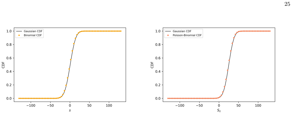
The load-bearing object is the signature $S_{ij}=C_{ij}-D_{ij}$, where $C_{ij}$ counts concordant dyadic motifs ($++$, $--$, and in the zero-inflated scheme also $00$) and $D_{ij}$ counts discordant motifs ($+-$, $-+$, and the partial motifs $0+$, $+0$, $0-$, $-0$). Under the maximum-entropy null models, each motif is a Bernoulli variable, making $S_{ij}$ Poisson-binomial for local constraints (BiSCM, BiSCM-FT) and binomial for global constraints (BiSRGM, BiSRGM-FT); the two-sided p-value follows from the cumulative distribution, and the false-discovery-rate procedure [58] converts the p-value matrix into a validated edge set. The zero-deflated schemes fix the bipartite topology and randomize only signs; the zero-inflated schemes leave topology free and count missing ties as part of concordance or discordance.
What would settle it
Generate signed bipartite networks from a null model with no community or block structure, run the full pipeline many times, and count the fraction of validated positive and negative edges; if that fraction consistently exceeds the 0.05 false-discovery-rate level, the p-value construction in Eqs. (33), (40), and (41) is miscalibrated.
Extended reading notes
Core claim
The paper's central claim is that a statistically validated projection of any binary undirected bipartite signed network can be obtained by defining, for each pair of nodes in the layer of interest, the signature $S_{ij}=C_{ij}-D_{ij}$, the difference between concordant and discordant shared motifs, and retaining a positive (negative) edge exactly when the empirical signature is so far from the benchmark expectation that the two-sided p-value $p_{ij}=2\min\{F(S^*_{ij}),1-F(S^*_{ij})\}$ falls below the FDR threshold. This is an unsupervised, white-box rule: no hand-tuned threshold is needed, and the output is a matrix of link-specific p-values from which the projection follows. The authors test the algorithm on synthetic block-model configurations and on U.S. Senate, U.S. House, and FilmTrust data, finding modules that survive validation and are not explained by the constraints encoded in the benchmarks.
Load-bearing premise
The load-bearing premise is that each sign and each missing link can be treated as an independent random variable once its probability is fitted from the data, and that the false-discovery-rate correction still controls errors when the pairwise tests are correlated and the number of tested hypotheses is counted through shared motifs rather than through node pairs.
Editorial extensions
If this is right
- Validated projections are sparser than naive ones: the local filters cut more edges than the global filter on all three real-world datasets, and both filters reveal more BIC-detected modules than the naive projections.
- The surviving structures favor relaxed balance theory: negative links appear inside modules and positive links between modules in several projections, a pattern traditional balance theory rules out.
- The algorithm doubles as a sign-prediction rule: pairs with significantly concordant motifs get +1, significantly discordant pairs get -1, and non-significant pairs are left unlinked.
- Because the output is a p-value matrix, any multiple-hypothesis procedure can be swapped in place of the FDR filter without changing the earlier steps.
Reading between the lines
- Setting the FDR denominator to $|H|=\sum_{i<j} V_{ij}$ in the zero-deflated scheme, rather than to the number of tested node pairs $N(N-1)/2$, may make the threshold less conservative; recomputing the Senate and House projections with the full denominator would show whether the detected modules survive.
- The zero-inflated treatment of a $00$ motif as concordance encodes a substantive assumption about missingness; an analysis that instead treats missing ties as neutral would test how much of the "self-organisation" reading depends on that choice.
- The same p-value machinery could be applied to temporal signed bipartite data to ask whether validated agreement/disagreement networks become more balanced over time, a prediction the paper's cross-sectional results hint at but do not test.
Editorial analysis
A structured set of objections, weighed in public.
Referee Report
Summary. The paper proposes a method for obtaining statistically validated signed projections of binary undirected bipartite signed networks. Two schemes are defined: a zero-deflated scheme that ignores motifs involving missing ties and a zero-inflated scheme that treats missing ties as agreeing/disagreeing evidence. For each node pair, a signature S_ij is compared with its distribution under maximum-entropy benchmarks (global and local, fixed- and free-topology variants, namely BiSRGM-FT, BiSCM-FT, BiSRGM, BiSCM), yielding a two-sided p-value from a binomial or Poisson-binomial distribution. The p-value matrix is thresholded with the Benjamini-Hochberg FDR procedure to produce positive/negative/zero edges in the projection. The method is tested on synthetic BiSSBM configurations and applied to FilmTrust, U.S. Senate, and U.S. House of Representatives data, where the authors claim to detect non-trivial mesoscopic structures that reveal 'genuine traces of self-organisation'.
Significance. The paper addresses a genuine gap: statistically validated projections for signed bipartite networks are much less developed than for unsigned networks. The derivations in Appendices A and B are careful and internally consistent, the synthetic tests based on a fully controllable generative model are appropriate, and the authors release their code. If the multiple-testing step is correctly calibrated, the proposed tool would be a useful contribution to the statistical validation of signed bipartite projections. However, the current FDR implementation contains two load-bearing problems, so the 'statistically validated' claim in the abstract is not yet supported as written.
major comments (3)
- [Appendix C and Section IV.H] The definition of |H| in Appendix C is inconsistent with the procedure that actually generates the p-values. Step B of Section IV.E computes one p-value per node pair, yet Appendix C sets |H| = sum_{i<j} V_ij within the zero-deflated scheme. The BH procedure requires |H| to be the number of p-values in the sorted list; if the actual list has length m, the critical value for the i-th sorted p-value is i*t/m. Using sum_{i<j} V_ij instead of m (or instead of the number of pairs with V_ij>0, if zero-common-neighbour pairs are excluded) changes the rejection threshold and invalidates the claimed FDR control. Depending on the data, sum_{i<j} V_ij can be larger or smaller than the number of tested pairs, so the miscalibration can be either conservative or anti-conservative. Please correct |H| to the actual number of tested hypotheses and explicitly state how pairs with V_ij=0 are handled.
- [Section IV.H] The statement that FDR controls errors 'irrespectively of the independence of the hypotheses tested' is not correct for the Benjamini-Hochberg procedure. BH controls FDR under independence or under positive regression dependence (PRDS), but not under arbitrary dependence. The p-values produced here are dependent: S_ij and S_ik are functions of the same signed entries b_iα for common items α, and the manuscript supplies no PRDS proof and no dependence-robust correction. A concrete fix is to prove the required dependence property for these p-values, to replace BH with a dependence-robust method (e.g., Benjamini-Yekutieli), or to calibrate the procedure by simulation under the null model.
- [Section II.B.2-3] The real-world mesoscopic conclusions, including the claim of 'genuine traces of self-organisation', are drawn from the edge sets produced by the FDR step. These conclusions therefore inherit the FDR calibration problems described above. Once the multiple-testing step is corrected, the corresponding claims about modular structures, negative/positive modules, and balance-theory alignment should be re-examined, since the validated edge set may change.
minor comments (4)
- [Appendix E, Eq. (E2)] The update equation for y_i has a typo: the numerator should be w_alpha^{(n-1)}, not z_alpha^{(n-1)}, to match the derivative with respect to y_i. The same typo appears in the displayed iterative form.
- [Table I] The fourth row is labelled 'Zero-deflated projection - nai¨ve' but, based on its values and the surrounding rows, it should be labelled 'Zero-inflated projection - nai¨ve'. In addition, the entry '1.135.278' appears to be a malformed number.
- [Appendix E, Eq. (E8)] The definition of MRE uses expressions such as |k^-_i(B*)⟨k^-_i⟩| / k^-_i(B*), which are missing the subtraction operator; it should read |k^-_i(B*) - ⟨k^-_i⟩| / k^-_i(B*), and analogously for the h^-_alpha term.
- [Section IV.G.1] The text 'see Sections IV I 1, IV I 1' contains a duplicated cross-reference; one of the two references appears to be intended for the local-constraint model and the other for the global-constraint model.
Circularity Check
No significant circularity: the validated projection is derived from a null model calibrated on the data, and the central claims are tested against independently generated synthetic configurations.
full rationale
The paper's derivation chain is self-contained in the relevant sense. The similarity S_ij is computed directly from the empirical biadjacency matrix, the null distributions for S_ij are derived from maximum-entropy benchmarks whose parameters are fitted to the observed network, and the resulting p-values are then thresholded with a multiple-hypothesis procedure. None of these steps inserts the target conclusion—that certain concordant or discordant co-occurrences are statistically significant—into the input. The synthetic validation is genuinely independent: the BiSSBM generative model is defined by user-chosen probabilities, configurations are generated from it, and the projection algorithm's output is compared with the known planted structure. Self-citations appear (e.g., the BiSRGM/BiSCM benchmarks from earlier work by the same group and the BIC-based partitioning recipe), but the benchmarks are re-derived within the paper itself and the partitioning recipe is used only for descriptive mesoscale analysis, not as the justification for the projection. The FDR-related concerns raised by a skeptical reader—that Benjamini-Hochberg is invoked while the p-values are dependent and that Appendix C sets |H| to sum V_ij rather than the number of tested node pairs—are validity and calibration issues, not circularity: they question whether the stated error-control guarantee applies, not whether the output reduces by construction to an input. Accordingly, no circular step can be exhibited with the required specificity, and the honest finding is no significant circularity.
Assumptions & free parameters
free parameters (5)
- FDR single-test significance level t =
0.05
- BiSRGM-FT positive-link probability p+ =
L+ / L per dataset
- BiSRGM probabilities p+, p- =
L+ / (N M), L- / (N M)
- BiSCM and BiSCM-FT Lagrange multipliers =
Numeric, one set per dataset
- Number of SSBM blocks k =
varies per projection, 2 to 32
assumptions (4)
- domain assumption Link variables are independent under the null benchmarks
- standard math Maximum-entropy exponential random graphs are the appropriate null family
- domain assumption Benjamini-Hochberg FDR controls error for dependent pairwise p-values
- ad hoc to paper Both nodes missing an item counts as agreement (zero-inflated scheme)
Cite this review
Pith. "Pith review of Statistically validated projection of bipartite signed networks." pith.science (2026). https://pith.science/paper/5ZHK457M
@misc{pith2026250208567,
  author       = {Pith},
  title        = {Pith review of: Statistically validated projection of bipartite signed networks},
  year         = {2026},
  howpublished = {\url{https://pith.science/paper/5ZHK457M}},
  note         = {Machine review of arXiv:2502.08567}
}
abstract
Bipartite networks provide a major insight into the organisation of many real-world systems. One of the most relevant issues encountered when modelling a bipartite network is that of facing the information shortage concerning intra-layer linkages. In the present contribution, we propose an unsupervised algorithm to obtain statistically validated projections of bipartite signed networks, according to which any two nodes sharing a statistically significant number of concordant (discordant) relationships are connected by a positive (negative) edge. Our algorithm outputs a matrix of link-specific $p-$values, from which a validated projection can be obtained upon running a multiple-hypothesis testing procedure. After testing our method on synthetic configurations output by a fully controllable generative model, we apply it to several real-world configurations: in all cases, non-trivial mesoscopic structures, induced by relationships that cannot be traced back to the constraints defining the employed benchmarks, hence revealing genuine traces of self-organisation, are detected.
Figures


Figures from the paper (6 more)


Reference graph
Works this paper leans on
-
[1]
When considering the unsigned case, the link density of the projection returned by the na ¨ ıve approach is typi- cally large [36]
Na ¨ ıve projection of real-world configurations The aforementioned configurations have been, first, na ¨ ıvely projected according to the recipes ana ¨ ıve ij = sgn[Sij], valid within the zero-deflated scheme, and ana ¨ ıve ij = sgn[Sij], valid within the zero-inflated scheme. When considering the unsigned case, the link density of the projection returne...
-
[2]
For what concerns U.S
Validated projection of real-world configurations within the zero-deflated scheme Although summing motifs while retaining their own sign is, in a sense, enough to obtain sparse projections, the validation procedure proposed in this paper (also) aims at enhancing the identification of patterns encoding non-trivial information about the original structure. ...
-
[3]
Validated projection of real-world configurations within the zero-inflated scheme The considerations above are confirmed by the zero- inflated projections depicted in Fig. 3. For example, pro- gressively filtering FilmTrust leads from a fully connected network to configurations whose connectance practically halves at each step. More in detail, applying th...
-
[4]
Zero-deflated projection scheme The first step of our method prescribes to measure the degree of similarity of nodes i and j. To this aim, let us consider the quantity named signature and defined as: Sij = VijX α=1 biαbjα = VijX α=1 [(b+ iαb+ jα + b− iαb− jα) − (b+ iαb− jα + b− iαb+ jα)] = VijX α=1 (Cijα − Dijα) = Cij − Dij (22) where the sum runs over th...
-
[5]
Zero-inflated projection scheme Let us, now, measure the degree of similarity of nodes i and j within the zero-inflated projection scheme. To this aim, let us consider the novel definition of signature reading Sij = MX α=1 (Cijα − Dijα) = Cij − Dij (26) where the concordance between nodes i and j, now, reads Cij = MX α=1 Cijα = V ++ ij + V −− ij + V 00 ij...
-
[6]
Zero-deflated projection scheme The second step of our method prescribes to evaluate the statistical significance of our nodes similarity. To this aim, let us find the probability distribution obeyed by Sij, after noticing that −Vij ≤ Sij ≤ Vij (30) where Sij = −Vij if Cij = 0 (i.e. if each ‘full’ V-motif is composed by a −1 and a +1) and Sij = Vij if Dij...
-
[7]
if each V-motif is composed by a −1 and a +1) and Sij = M if Dij = 0 (i.e
Zero-inflated projection scheme Let us, now, find the probability distribution obeyed by Sij, after noticing that −M ≤ Sij ≤ M (34) where Sij = −M if Cij = 0 (i.e. if each V-motif is composed by a −1 and a +1) and Sij = M if Dij = 0 (i.e. if each V-motif is composed by either two −1s or two +1s). As in the previous subsection, let us treat links link as i...
-
[8]
In what follows we will focus on Sij but the same considerations hold true for Sij
Quantifying the statistical significance of similarity Once we have calculated the distribution for each pair of nodes belonging to the layer of interest, we have to calculate the statistical significance of the empirical sig- nature: as we have a signed quantity, we need both tails of such a distribution to carry out what is known as two- sided test of h...
Show all 85 references
-
[9]
Zero-deflated projection scheme The first two benchmarks determine the coefficients of the two variants of the finite scheme defined in Eq. 31. As already stressed, dyadic motifs constituted by, at least, one missing tie are ignored, here: the bipartite topology is, thus, cons...
-
[10]
Zero-inflated projection scheme The other two benchmarks determine the coefficients of the two variants of the finite scheme defined in Eq. 35. As already stressed, dyadic motifs constituted by, at least, one missing tie are accounted for, here: the bipartite topology is, thus...
2022
-
[11]
Antal, P
T. Antal, P. L. Krapivsky, and S. Redner, Physica D: Nonlinear Phenomena 224, 130 (2006)
2006
-
[12]
Leskovec, D
J. Leskovec, D. Huttenlocher, and J. Kleinberg, in Pro- ceedings of the SIGCHI Conference on Human Factors in Computing Systems (2010) pp. 1361–1370
2010
-
[13]
Zaslavsky, The Electronic Journal of Combinatorics , DS8 (2012)
T. Zaslavsky, The Electronic Journal of Combinatorics , DS8 (2012)
2012
-
[14]
J. Tang, Y. Chang, C. Aggarwal, and H. Liu, ACM Computing Surveys (CSUR) 49, 1 (2016)
2016
-
[15]
Heider, The Journal of Psychology 21, 107 (1946)
F. Heider, The Journal of Psychology 21, 107 (1946)
1946
-
[16]
Cartwright and F
D. Cartwright and F. Harary, Psychological Review 63, 277 (1956)
1956
-
[17]
J. A. Davis, Human Relations 20, 181 (1967)
1967
-
[18]
Gallo, D
A. Gallo, D. Garlaschelli, T. Squartini, et al. , Physical Review Research 6 (2024)
2024
-
[19]
Harary, M.-H
F. Harary, M.-H. Lim, and D. C. Wunsch, IMA Journal of Management Mathematics 13, 201 (2002)
2002
-
[20]
Ou-Yang, D.-Q
L. Ou-Yang, D.-Q. Dai, and X.-F. Zhang, IEEE/ACM Transactions on Computational Biology and Bioinfor- matics 12, 1333 (2015)
2015
-
[21]
Iorio, M
F. Iorio, M. Bernardo-Faura, A. Gobbi, T. Cokelaer, G. Jurman, and J. Saez-Rodriguez, BMC Bioinformatics 17, 1 (2016)
2016
-
[22]
H. Saiz, J. G´ omez-Garde˜ nes, P. Nuche, A. Gir´ on, Y. Pueyo, and C. L. Alados, Ecography 40, 733 (2017)
2017
-
[23]
Gallo, D
A. Gallo, D. Garlaschelli, R. Lambiotte, F. Saracco, and T. Squartini, Communications Physics 7, 154 (2024)
2024
-
[24]
Gallo, F
A. Gallo, F. Saracco, R. Lambiotte, D. Garlaschelli, and T. Squartini, Phys. Rev. E 111, 024312 (2025). 19
2025
-
[25]
Candellone, E.-J
E. Candellone, E.-J. van Kesteren, S. Chelmi, and J. Garcia-Bernardo, Advances in Complex Systems 28 (2025)
2025
-
[26]
Talaga, M
S. Talaga, M. Stella, T. J. Swanson, and A. S. Teixeira, Communication Physics 6 (2023)
2023
-
[27]
A. S. Teixeira, F. C. Santos, and A. P. Francisco, in International Workshop on Complex Networks (Springer,
-
[28]
Doreian and A
P. Doreian and A. Mrvar, Social Networks 31, 1 (2009)
2009
-
[29]
Mrvar and P
A. Mrvar and P. Doreian, Journal of Mathematical Soci- ology 33, 196 (2009)
2009
-
[30]
Derr and J
T. Derr and J. Tang, in 2018 IEEE International Con- ference on Data Mining Workshops (ICDMW) (IEEE,
2018
-
[31]
T. Derr, C. Johnson, Y. Chang, and J. Tang, in Proceed- ings of the 28th ACM International Conference on In- formation and Knowledge Management (2019) pp. 1221– 1230
2019
-
[32]
Saracco, R
F. Saracco, R. Di Clemente, A. Gabrielli, and T. Squar- tini, Scientific reports 5, 10595 (2015)
2015
-
[33]
Huang, H
J. Huang, H. Shen, Q. Cao, S. Tao, and X. Cheng, in Proceedings of the 30th ACM International Conference on Information & Knowledge Management (2021) pp. 740–749
2021
-
[34]
Banerjee, K
S. Banerjee, K. Sarkar, S. Gokalp, A. Sen, and H. Davulcu, in Social Computing, Behavioral-Cultural Modeling and Prediction: 5th International Conference, SBP 2012, College Park, MD, USA, April 3-5, 2012. Proceedings 5 (Springer, 2012) pp. 196–204
2012
-
[35]
Neal, Social Networks 39, 84 (2014)
Z. Neal, Social Networks 39, 84 (2014)
2014
-
[36]
Latapy, C
M. Latapy, C. Magnien, and N. Del Vecchio, Social net- works 30, 31 (2008)
2008
-
[37]
D. J. Watts and S. H. Strogatz, nature 393, 440 (1998)
1998
-
[38]
Derudder and P
B. Derudder and P. Taylor, Global Networks5, 71 (2005)
2005
-
[39]
M. ´A. Serrano, M. Bogun´ a, and A. Vespignani, Pro- ceedings of the national academy of sciences 106, 6483 (2009)
2009
-
[40]
Zaccaria, M
A. Zaccaria, M. Cristelli, A. Tacchella, and L. Pietronero, PloS one 9, e113770 (2014)
2014
-
[41]
Caldarelli, M
G. Caldarelli, M. Cristelli, A. Gabrielli, L. Pietronero, A. Scala, and A. Tacchella, PLoS ONE (2012)
2012
-
[42]
Linden, B
G. Linden, B. Smith, and J. York, IEEE Internet com- puting 7, 76 (2003)
2003
-
[43]
Bonacich, Journal of mathematical sociology 2, 113 (1972)
P. Bonacich, Journal of mathematical sociology 2, 113 (1972)
1972
-
[44]
Tumminello, S
M. Tumminello, S. Micciche, F. Lillo, J. Piilo, and R. N. Mantegna, PloS one 6, e17994 (2011)
2011
-
[45]
Gualdi, G
S. Gualdi, G. Cimini, K. Primicerio, R. Di Clemente, and D. Challet, Scientific reports 6, 39467 (2016)
2016
-
[46]
Saracco, M
F. Saracco, M. J. Straka, R. Di Clemente, A. Gabrielli, G. Caldarelli, and T. Squartini, New Journal of Physics 19, 053022 (2017)
2017
-
[47]
Dianati, arXiv preprint arXiv:1607.01735 (2016)
N. Dianati, arXiv preprint arXiv:1607.01735 (2016)
2016 arXiv
-
[48]
Z. P. Neal, Plos one 19, e0311614 (2024)
2024
-
[49]
Z. P. Neal, Social networks 60, 103 (2020)
2020
-
[50]
Z. P. Neal, A. Cadieux, D. Garlaschelli, N. J. Gotelli, F. Saracco, T. Squartini, S. T. Shutters, W. Ulrich, G. Wang, and G. Strona, PLOS Complex Systems 1, e0000010 (2024)
2024
-
[51]
L. Li, K. Gu, A. Zeng, Y. Fan, and Z. Di, Physica A: Sta- tistical Mechanics and its Applications 495, 345 (2018)
2018
-
[52]
Fouss, A
F. Fouss, A. Pirotte, J.-M. Renders, and M. Saerens, IEEE Transactions on knowledge and data engineering 19, 355 (2007)
2007
-
[53]
Baltakys, Scientific Reports 13, 1072 (2023)
K. Baltakys, Scientific Reports 13, 1072 (2023)
2023
-
[54]
Tracking the United States Congress,
“Tracking the United States Congress,”
-
[55]
G. Guo, J. Zhang, and N. Yorke-Smith, in Proc. Int. Joint Conf. on Artif. Intell. (2013) pp. 2619–2625
2013
-
[56]
Kunegis, in Proc
J. Kunegis, in Proc. Int. Conf. on World Wide Web Com- panion (2013) pp. 1343–1350
2013
-
[57]
Singh and B
R. Singh and B. Adhikari, Journal of Statistical Mechan- ics: Theory and Experiment 2017, 063302 (2017)
2017
-
[58]
Andres, G
G. Andres, G. Casiraghi, G. Vaccario, and F. Schweitzer, Scientific Reports 13, 20689 (2023)
2023
-
[59]
Dang and C.-L
Q.-V. Dang and C.-L. Ignat, in 2018 IEEE 4th interna- tional conference on collaboration and internet computing (CIC) (IEEE, 2018) pp. 36–45
2018
-
[60]
T. Derr, Y. Ma, and J. Tang, in 2018 IEEE International Conference on Data Mining (ICDM) (IEEE, 2018) pp. 929–934
2018
-
[61]
D. Li, D. Shen, Y. Kou, and T. Nie, IEEE Access 7, 171357 (2019)
2019
-
[62]
Zhang, J
Z. Zhang, J. Liu, K. Zhao, S. Yang, X. Zheng, and Y. Wang, in Proceedings of the 46th International ACM SIGIR Conference on Research and Development in In- formation Retrieval (2023) pp. 1629–1638
2023
-
[63]
Jiang, J
Y. Jiang, J. Yu, Z. Xu, C. Chen, Y.-W. Chow, and Y. Zhang, in Asia-Pacific Web (APWeb) and Web-Age Information Management (WAIM) Joint International Conference on Web and Big Data (Springer, 2024) pp. 81–96
2024
-
[64]
Psycho-logic, Attitude Change 3, 86 (1958)
S. Psycho-logic, Attitude Change 3, 86 (1958)
1958
-
[65]
Cartwright and F
D. Cartwright and F. Harary, Behavioral Science 15, 497 (1970)
1970
-
[66]
Schoch, The Journal of Mathematical Sociology 45, 37 (2021)
D. Schoch, The Journal of Mathematical Sociology 45, 37 (2021)
2021
-
[67]
A. Y. Khintchine, Mathematical foundations of informa- tion theory (Dover, 1957)
1957
-
[68]
Benjamini and Y
Y. Benjamini and Y. Hochberg, Journal of the Royal sta- tistical society: series B (Methodological) 57, 289 (1995)
1995
-
[69]
E. T. Jaynes, Physical review 106, 620 (1957)
1957
-
[70]
Park and M
J. Park and M. E. J. Newman, Physical Review E 70, 66117 (2004)
2004
-
[71]
Squartini and D
T. Squartini and D. Garlaschelli, New Journal of Physics 13, 083001 (2011)
2011
-
[72]
Squartini and D
T. Squartini and D. Garlaschelli, Maximum-Entropy Net- works. Pattern Detection, Network Reconstruction and Graph Combinatorics (Springer International Publish- ing, 2017) p. 116
2017
-
[73]
Cimini, T
G. Cimini, T. Squartini, F. Saracco, D. Garlaschelli, A. Gabrielli, and G. Caldarelli, Nature Reviews Physics 1, 58 (2018)
2018
-
[74]
Garlaschelli and M
D. Garlaschelli and M. I. Loffredo, Physical Review E 78, 1 (2008)
2008
-
[75]
Hao and I
B. Hao and I. A. Kov´ acs, Science Advances10, eadj0104 (2024)
2024
-
[76]
Vallarano, M
N. Vallarano, M. Bruno, E. Marchese, G. Trapani, F. Saracco, G. Cimini, M. Zanon, and T. Squartini, Sci- entific Reports 11, 15227 (2021)
2021
-
[77]
Becatti, G
C. Becatti, G. Caldarelli, and F. Saracco, Physical Re- view E 99, 022306 (2019). 20 Appendix A: The distribution of the signature in the zero-deflated scheme Let us, first, remind that such a scheme devises a recipe for projecting a bipartite network that ignores the V-motifs...
2019
-
[78]
|biα| = 1 (A1) and further inducing biαbjα ∼ −1 +1 2p+(1 − p+) 1 − 2p+ + 2(p+)2 = −1 +1 1 − q+ q+ , ∀ i, j, αs.t
Benchmarks with global constraints A benchmark with global constraints is defined by the finite scheme reading biα ∼ −1 +1 1 − p+ p+ , ∀ i, αs.t. |biα| = 1 (A1) and further inducing biαbjα ∼ −1 +1 2p+(1 − p+) 1 − 2p+ + 2(p+)2 = −1 +1 1 − q+ q+ , ∀ i, j, αs.t. |biαbjα| = 1; (A2...
-
[79]
|biα| = 1, (A10) further inducing biαbjα ∼ −1 +1 p+ iα + p+ jα − 2p+ iαp+ jα 1 − p+ iα − p+ jα + 2p+ iαp+ jα = −1 +1 1 − q+ ijα q+ ijα , ∀ i, j, αs.t
Benchmarks with local constraints A benchmark with local constraints is defined by the finite scheme reading biα ∼ −1 +1 1 − p+ iα p+ iα , ∀ i, αs.t. |biα| = 1, (A10) further inducing biαbjα ∼ −1 +1 p+ iα + p+ jα − 2p+ iαp+ jα 1 − p+ iα − p+ jα + 2p+ iαp+ jα = −1 +1 1 − q+ ijα...
-
[80]
Naturally, ⟨b+ iαb+ jα⟩ = q++ and Var[b+ iαb+ jα] = q++(1 − q++) and analogously for the other motifs
Benchmarks with global constraints A benchmark with global constraints is defined by the finite scheme reading biα ∼ −1 0 +1 p− p0 p+ , ∀ i, α (B1) that, in turn, leads to b+ iαb+ jα ∼ 0 +1 1 − (p+)2 (p+)2 = 0 +1 1 − q++ q++ , ∀ i, j, α, (B2) b− iαb− jα ∼ 0 +1 1 − (p−)2 (p−)2 ...
-
[81]
Benchmarks with local constraints A benchmark with local constraints is defined by the finite scheme reading Cijα = b+ iαb+ jα + b− iαb− jα + b0 iαb0 jα ∼ 0 +1 1 − q+ ijα q+ ijα , ∀ i, j, α, (B15) Dijα = b+ iαb− jα + b− iαb+ jα + b0 iαb+ jα + b+ iαb0 jα + b0 iαb− jα + b− iαb0 ...
-
[82]
Naturally, p0 = 1 − p− − p+
F ree-topology Bipartite Signed Random Graph Model (BiSRGM) The Hamiltonian describing such a problem reads H(θ, B) = βL+(B) + γL−(B) = NX i=1 MX α=1 (βb+ iα + γb− iα); (D3) as a consequence, the partition function reads Z(θ) = X B∈B NY i=1 MY α=1 e−(βb+ iα+γb− iα) = NY i=1 MY...
-
[83]
The Hamiltonian describing such a problem still reads H(θ, B) = β′L+(B) + γ′L−(B) = NX i=1 MX α=1 (β′b+ iα + γ′b− iα)
Fixed-topology Bipartite Signed Random Graph Model (BiSRGM-FT) Let us, again, consider the properties L+(B) and L−(B), to be satisfied by keeping a bipartite network topology fixed. The Hamiltonian describing such a problem still reads H(θ, B) = β′L+(B) + γ′L−(B) = NX i=1 MX α...
-
[84]
The Hamiltonian describing such a problem reads H(θ, B) = NX i=1 [βik+ i (B) + γik− i (B)] + MX α=1 [δαh+ α (B) + ηαh− α (B)]
F ree-topology Bipartite Signed Configuration Model (BiSCM) The second set of constraints we consider is represented by the properties {k+ i (B)}N i=1, {k− i (B)}N i=1, {h+ α (B)}M α=1 and {h− α (B)}M α=1. The Hamiltonian describing such a problem reads H(θ, B) = NX i=1 [βik+ ...
-
[85]
Fixed-topology Bipartite Signed Configuration Model (BiSCM-FT) Let us, again, consider the properties {k+ i (B)}N i=1, {k− i (B)}N i=1, {h+ α (B)}M α=1 and {h− α (B)}M α=1 to be satisfied by keeping a bipartite network topology fixed. The Hamiltonian describing such a problem ...
Reviewed August 8, 2026 · model on record in the stance chip above.
Discussion (0). Continue with ORCID to comment.