REVIEW 4 major objections 5 minor 59 references
A Deep Learning approach for parametrized and time dependent Partial Differential Equations using Dimensionality Reduction and Neural ODEs
T0 review · 4 major / 5 minor · reviewed 2026-08-08 · deepseek-v4-flash
Pith's one-line read Dimensionality reduction plus a latent Neural ODE gives a surrogate for time-dependent parametric PDEs that is more accurate, two times lighter, and two times faster than state-of-the-art neural models.
desk verdict Solid empirical recipe for latent-ODE surrogates; the L3 consistency loss and the TF/AR training schedule are the real novelties, but the benchmark comparisons need error bars and the closest latent-ODE baselines. read the letter →
The pith
A machine-rendered reading of the paper's core claim, the machinery that carries it, and where it could break.
The reading
What carries the argument
The load-bearing mechanism is the coupling of an autoencoder with a latent Neural ODE. The encoder $\varphi_\theta$ and decoder $\psi_\theta$ map between the discretized solution space $S_r$ and a latent space $E$ of dimension $\lambda$ far smaller than the full discretized field dimension, and the processor $\pi_\theta$ advances a latent vector by numerically integrating the latent ODE $\frac{d}{dt}\varepsilon(t|\boldsymbol{\mu}) = f_\theta(\varepsilon(t|\boldsymbol{\mu}),\boldsymbol{\mu})$ with a Runge–Kutta scheme of stage $q$ (typically 4). The identity that carries the argument is step-size coherence: because $\pi_\theta$ takes $\Delta t$ as an input, the same learned $f_\theta$ must give consistent rollouts for different time steps, and the training enforces this only softly through the loss $L_3$ of Equation (14), which advances the latent state through a randomly sampled intermediate time step in $[0,\Delta t]$. Appendix A.1 shows why the Runge–Kutta stage matters: under Euler integration, exact coherence forces $f_\theta$ to be constant (Equation 20), while a second-order scheme already permits a nontrivial vector field (Equation 24), so higher-stage integrators improve both accuracy and time generalization. The full training objective combines the reconstruction loss $L_1$, a teacher-forcing term, an autoregressive term with truncated backpropagation through time, and $L_3$; the varying-parameter experiments require the autoregressive term to be ramped in gradually during training.
What would settle it
Retrain the comparison models on the exact same PDEBench data, training time steps, and train/validation/test splits used for the proposed model, and evaluate all models on the same test grids; if the accuracy, weight, and speed advantages do not survive, the central claim fails. A complementary calculation for the underlying assumption: for a model trained with Euler integration, check whether the learned vector field satisfies $f_\theta(\varepsilon(t_i)) = f_\theta(\varepsilon(t_m))$ at intermediate states, since the paper's Equation (20) requires exact equality for full step-size coherence, and any measurable violation bounds the claimed time generalization.
Extended reading notes
Core claim
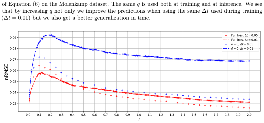
The authors claim that the solution operator of a time-dependent, parameter-dependent PDE can be learned by mapping each high-fidelity solution field into a low-dimensional latent vector with an autoencoder and then evolving that vector with a Neural ODE, $\frac{d}{dt}\varepsilon(t|\boldsymbol{\mu}) = f_\theta(\varepsilon(t|\boldsymbol{\mu}),\boldsymbol{\mu})$, whose vector field is a small network conditioned on the PDE parameters. Because the latent dynamics are continuous in time and the processor $\pi_\theta$ takes the time step $\Delta t$ as an input, a model trained on one time step can be run at finer time steps at inference. Trained with a combination of a reconstruction loss, a teacher-forced one-step prediction loss, an autoregressive rollout loss with truncated backpropagation, and an intermediate-time-step loss $L_3$, the model reports lower normalized root-mean-square error (nRMSE) than FNO, MP-PDE, U-Net, CORAL, OFormer, Galerkin, and VCNeF on the 1D Advection and 1D Burgers benchmarks, lower nRMSE than FNO, U-Net, and PINN on the 2D Shallow Water equations despite being trained on coarser time steps, and lower nRMSE over time than VCNeF on the 2D Molenkamp test, while using at least two times fewer parameters and running at least two times faster at inference. The authors read these results as evidence that dimensionality reduction, rather than larger and more complex architectures, is the key to fast and memory-efficient surrogates for repeated PDE solves. They also note that generalization to parameters outside the training range remains partial for the advection and Burgers cases, which they attribute to the choice of training parameter points.
Load-bearing premise
The method assumes that the low-dimensional latent state truly follows a single autonomous ordinary differential equation, and that the same learned function stays consistent when the time step changes; the training enforces this consistency only through a soft loss term, and the paper itself shows that exact consistency would force the learned function to be constant for the simplest integrator.
Editorial extensions
If this is right
- Accurate surrogates for time-dependent parametric PDEs need not be large: the reported results put a model with roughly 167–217 thousand weights below competitors with 530 thousand to 1.6 million weights on nRMSE, so memory-limited deployments become realistic.
- A model trained at $\Delta t = 0.05$ s can be rolled out at $\Delta t = 0.01$ s with almost no error increase, so a single training run serves multiple temporal resolutions and users can take larger latent steps during routine repeated evaluations.
- Higher-stage Runge–Kutta solvers inside the latent ODE improve both accuracy and time generalization according to the ablation experiments, making the choice of latent integrator a modeling decision rather than an implementation detail.
- The training recipe that combines teacher forcing with a gradually ramped autoregressive term is what makes the method work for varying-parameter PDEs, and it transfers as a strategy to other latent-dynamics surrogates.
- Because the latent ODE is continuous in time, the trained surrogate can be queried at arbitrary intermediate times without retraining, in contrast to models that only predict at fixed discrete steps.
Reading between the lines
- Because step-size coherence is only softly enforced, the claimed time generalization should have a limit: below some $\Delta t$ far outside the range sampled by $L_3$, or for stiff latent dynamics, rollout error would grow non-smoothly; a testable extension is to bias $L_3$'s random intermediate steps toward very small $\Delta t$ and measure whether finer-time generalization improves.
- The convolutional encoder and decoder, which the authors name as the main limitation, tie the method to a fixed grid; replacing them with a discretization-agnostic map would carry the latent-ODE recipe to unstructured and dynamically changing meshes without retraining.
- The comparison is against deep-learning surrogates only; a head-to-head with classical POD-based reduced-order models on the same benchmarks would test whether the advantage comes from the learned nonlinear manifold rather than from reduced-order modeling per se.
- Because the method trains on coarser time steps, each trajectory needs fewer stored time slices, so a cost advantage plausibly extends to training data and training time, although the paper only claims inference-time savings.
Editorial analysis
A structured set of objections, weighed in public.
Referee Report
Summary. The paper proposes an autoregressive surrogate model for time-dependent, parametric PDEs. A convolutional autoencoder maps full-order solution fields into a low-dimensional latent space, a small MLP defines a latent Neural ODE that advances latent states through a Runge-Kutta integrator, and the decoder maps latent states back to physical fields. Training uses a reconstruction loss, a teacher-forcing latent loss, an autoregressive truncated-BPTT latent loss, and an additional time-split consistency loss L3 intended to promote generalization to finer time steps. The method is benchmarked on 1D advection, 1D Burgers, 2D shallow-water, and 2D Molenkamp problems from PDEBench and compared with FNO, MP-PDE, UNet, CORAL, Galerkin, OFormer, VCNeF, and PINN results taken from the literature. The central claim is that dimensionality reduction yields a lighter, faster, and more accurate model than existing neural-operator approaches, with the additional ability to train on one time step and evaluate on a finer time step.
Significance. If the results hold, the paper provides a practically useful demonstration that a small autoencoder plus latent NODE can outperform much larger neural operators on standard PDE benchmarks, with direct relevance to uncertainty quantification and design optimization. The manuscript is strong on reproducibility-oriented detail: Appendix C lists hyperparameters and training schedules, Appendix B gives full architecture specifications, and the ablation studies in Figures 7-10 directly probe the role of the Runge-Kutta stage and the L3 loss in time generalization. The L3 time-splitting idea is a simple and potentially transferable training technique. The main weaknesses are that accuracy results are single-run point estimates without uncertainty quantification, the shallow-water comparison mixes training temporal resolutions in a way that is difficult to interpret, and fine-time-step generalization is enforced only by a soft penalty rather than by an exact structural property, so the general claim needs to be scoped to the tested benchmarks.
major comments (4)
- [§3.1, Tables 1-2; §3.2, Figures 3-5] All nRMSE values are reported as single point estimates with no standard deviations or repeated-seed averaging. Because the claimed accuracy advantages over FNO, UNet, and VCNeF are often small (e.g., 0.0066 vs 0.0079 for 1D advection in Table 1), run-to-run variation could change the ranking. Please report mean and standard deviation over at least three to five seeds for the proposed method, and state explicitly which baseline numbers are fixed published values and which were rerun by the authors.
- [§3.1, Table 2; Appendix F.3] The 2D shallow-water comparison is not a controlled experiment: the proposed model is trained on 21 temporal snapshots at Δt=0.05 s, while FNO, U-Net, and PINN are trained on 101 snapshots at Δt=0.01 s. The table caption is also confusing because the header 'nRMSE, Δt=0.01 s' appears twice, and the caption says the gray column is the training Δt while the text says the same-number-of-timesteps comparison is between our white column and the other methods' gray column. The authors should clarify the exact comparison protocol and, ideally, add a baseline trained with the same 21-snapshot temporal resolution.
- [§2.6, Eq. (14); Appendix A.1, Eqs. (20),(24)] The time-generalization claim is supported only empirically, not by the model construction. Appendix A.1 itself shows that exact step-size consistency forces f_theta to be constant for Euler integration (Eq. 20) and imposes a strong constraint for RK2 (Eq. 24); for the RK4 scheme actually used, no analogous exact condition is derived, and the L3 loss samples only one random intermediate split per training step. The fine-Δt results in Tables 1-2 and Figures 5-10 are therefore dataset-specific observations. Either provide a consistency or error bound for RK4 in terms of the L3 residual, or explicitly reframe the contribution as 'generalizes on the tested benchmarks' rather than 'can generalize to any finer Δt.'
- [§3.3, Table 5; Appendix C.5] The 'at least 2 times faster' claim is based on a single dataset (Burgers with ν=0.001) and compares inference times measured on different GPUs (A100 PCIe for the proposed method versus A100-SXM4 for the published numbers from [23]). It is unclear whether the same batch size, time horizon, and evaluation protocol were used for all methods. The lighter-weight claim from Table 6 is more robust, but the speed claim should be scoped to the specific benchmark and hardware or measured on the same GPU with a common protocol.
minor comments (5)
- [Table 2 caption] The column header 'nRMSE, Δt = 0.01 s' is duplicated, making the intended gray/white comparison hard to parse; one column header should be labeled consistently with the caption text.
- [Table 5] There is a formatting error in the row 'Ours 932.43136.588' which appears to be missing a '±', and the row 'Ours 1846.729±270.72' has a suspicious extra digit; these should be proofread.
- [§2.4, citation [8]] The sentence about teacher forcing causing distribution shift cites reference [8], which is the Message Passing Neural PDE Solver paper; a standard sequence-to-sequence or teacher-forcing reference would be more appropriate here.
- [Table 6 caption] The caption says 'for ζ = 0.01/ζ varying' but ζ = 0.01 is not used for advection; this should presumably read 'ζ = 0.1 / ζ varying' or similar.
- [Figure 6 and §2.6] The figure would benefit from axis labels and a short caption explaining how the red training points and green finer-inference points relate to the dotted latent trajectory; currently the relation is difficult to read from the figure alone.
Circularity Check
No substantive circularity: predictions are genuinely held-out, and the time-step generalization is soft-enforced but empirically tested rather than derived from the inputs.
full rationale
The paper's central pipeline is an autoencoder mapping PDE states to a latent space, plus a latent neural ODE advanced by a Runge-Kutta integrator. The predicted fields are computed as psi_theta(pi_theta(...pi_theta(phi_theta(s0))...)), and the losses in Equations (11)-(14) are trained on PDEBench data with held-out initial conditions and parameters. None of these predictions is a fitted quantity renamed as a prediction: the test sets, error metrics, and comparison numbers in Tables 1-2 and Figures 3-5 are external or held out from the training data. The time-generalization claim is the only item that deserves scrutiny, but it is not circular. The paper explicitly derives in Appendix A.1 that exact step-size coherence under Euler would force f_theta to be constant (Equation 20) and under RK2 imposes the constraint of Equation (24); since the model uses RK4 and only enforces coherence through the soft loss L3 (Equation 14), the fine-Delta-t improvements are empirical observations on the tested benchmarks, not consequences of an identity. This is a soundness or robustness limitation, not a reduction of the prediction to its inputs. The only self-citations are reference [2], used for Molenkamp parameter ranges, and reference [47], cited for the general motivation of uncertainty quantification; neither carries the paper's load-bearing claims, and neither is used to forbid alternatives or to justify the latent-ODE ansatz. The latent ODE is an explicit modeling assumption, not a result derived from a self-citation chain. No equation in the manuscript makes a predicted output equal to a training target by construction, so no circular step can be exhibited.
Assumptions & free parameters
free parameters (5)
- latent dimension λ =
30 (advection, Burgers, parametric advection, parametric Burgers), 20 (shallow water), 50 (Molenkamp)
- f_theta network width and depth =
2 hidden layers x 50 neurons (fixed advection, shallow water), 4 x 200 (Burgers and parametric variants), 2 x 100…
- loss weights α, β, γ, δ and λ_rg =
Strategy 1: β=1, γ=0; Strategy 2: β=1, γ=1 with warm-up γ0=1/500 or 1/1000; δ not explicitly stated; λ_rg=0.0 or 0.001
- Runge-Kutta stage q =
4 (default)
- k2 schedule for truncated BPTT =
k2 starts at 1 and increases by 1 every 30 epochs
assumptions (4)
- domain assumption The high-fidelity solution space can be mapped nearly bijectively to a low-dimensional latent space by an autoencoder.
- domain assumption Latent trajectories evolve according to an autonomous ODE with no explicit time dependence: d/dt ε = f(ε, μ).
- ad hoc to paper A single learned f_theta can advance the latent state coherently for any step size, so that composing two small steps matches one large step.
- domain assumption The PDEBench solver solutions used as training and testing labels are sufficiently accurate references.
Cite this review
Pith. "Pith review of A Deep Learning approach for parametrized and time dependent Partial Differential Equations using Dimensionality Reduction and Neural ODEs." pith.science (2026). https://pith.science/paper/MYCFOUGM
@misc{pith2026250208683,
  author       = {Pith},
  title        = {Pith review of: A Deep Learning approach for parametrized and time dependent Partial Differential Equations using Dimensionality Reduction and Neural ODEs},
  year         = {2026},
  howpublished = {\url{https://pith.science/paper/MYCFOUGM}},
  note         = {Machine review of arXiv:2502.08683}
}
read the original abstract
Partial Differential Equations (PDEs) are central to science and engineering. Since solving them is computationally expensive, a lot of effort has been put into approximating their solution operator via both traditional and recently increasingly Deep Learning (DL) techniques. A conclusive methodology capable of accounting both for (continuous) time and parameter dependency in such DL models however is still lacking. In this paper, we propose an autoregressive and data-driven method using the analogy with classical numerical solvers for time-dependent, parametric and (typically) nonlinear PDEs. We present how Dimensionality Reduction (DR) can be coupled with Neural Ordinary Differential Equations (NODEs) in order to learn the solution operator of arbitrary PDEs. The idea of our work is that it is possible to map the high-fidelity (i.e., high-dimensional) PDE solution space into a reduced (low-dimensional) space, which subsequently exhibits dynamics governed by a (latent) Ordinary Differential Equation (ODE). Solving this (easier) ODE in the reduced space allows avoiding solving the PDE in the high-dimensional solution space, thus decreasing the computational burden for repeated calculations for e.g., uncertainty quantification or design optimization purposes. The main outcome of this work is the importance of exploiting DR as opposed to the recent trend of building large and complex architectures: we show that by leveraging DR we can deliver not only more accurate predictions, but also a considerably lighter and faster DL model compared to existing methodologies.
Figures


Figures from the paper (11 more)




Reference graph
Works this paper leans on
-
[35]
Space-time continuous pde forecasting using equivariant neural fields
David M Knigge, David R Wessels, Riccardo Valperga, Samuele Papa, Jan-Jakob Sonke, Efstratios Gavves, and Erik J Bekkers. Space-time continuous pde forecasting using equivariant neural fields. arXiv preprint arXiv:2406.06660 , 2024
arXiv 2024
-
[58]
Continuous PDE dynamics forecasting with implicit neural representations
Yuan Yin, Matthieu Kirchmeyer, Jean-Yves Franceschi, Alain Rakotomamonjy, and patrick gallinari. Continuous PDE dynamics forecasting with implicit neural representations. In The Eleventh International Conference on Learning Representations , 2023. 14 Appendix A Runge-Kutta schemes Runge-Kutta methods [ 3] are a family of numerical methods for the solution...
work page 2023
- [39]
-
[23]
Jan Hagnberger, Marimuthu Kalimuthu, Daniel Musekamp, and Mathias Niepert. Vectorized Conditional Neural Fields: A framework for solving time-dependent parametric partial differential equations. In Ruslan Salakhutdinov, Zico Kolter, Katherine Heller, Adrian Weller, Nuria Oliver, Jonathan Scarlett, and Felix Berkenkamp, editors, Proceedings of the 41st Int...
work page 2024
-
[1]
Christopher Aicher, Nicholas J. Foti, and Emily B. Fox. Adaptively truncating backpropagation through time to control gradient bias. In Ryan P. Adams and Vibhav Gogate, editors, Proceedings of The 35th Uncertainty in Artificial Intelligence Conference , volume 115 of Proceedings of Machine Learning Research, pages 799–808. PMLR, 22–25 Jul 2020
work page 2020
-
[2]
Fahad Alsayyari, Zolt´ an Perk´ o, Marco Tiberga, Jan Leen Kloosterman, and Danny Lathouwers. A fully adaptive nonintrusive reduced-order modelling approach for parametrized time-dependent problems. Computer Methods in Applied Mechanics and Engineering , 373:113483, January 2021
work page 2021
-
[3]
Uri M. Ascher and Linda R. Petzold. Computer methods for ordinary differential equations and differential-algebraic equations. 1998
work page 1998
-
[4]
Jimmy Lei Ba. Layer normalization. arXiv preprint arXiv:1607.06450 , 2016
arXiv 2016
Show all 59 references
-
[5]
Are neural operators really neural operators? frame theory meets operator learning
Francesca Bartolucci, Emmanuel de B´ ezenac, Bogdan Raoni´ c, Roberto Molinaro, Siddhartha Mishra, and Rima Alaifari. Are neural operators really neural operators? frame theory meets operator learning. arXiv preprint arXiv:2305.19913 , 2023
2023 arXiv
-
[6]
Representation equivalent neural operators: a framework for alias-free operator learning
Francesca Bartolucci, Emmanuel de Bezenac, Bogdan Raonic, Roberto Molinaro, Siddhartha Mishra, and Rima Alaifari. Representation equivalent neural operators: a framework for alias-free operator learning. In Thirty-seventh Conference on Neural Information Processing Systems , 2023
2023
-
[7]
Model reduction and neural networks for parametric pdes
Kaushik Bhattacharya, Bamdad Hosseini, Nikola B Kovachki, and Andrew M Stuart. Model reduction and neural networks for parametric pdes. The SMAI journal of computational mathematics , 7:121–157, 2021
2021
-
[8]
Message passing neural pde solvers
Johannes Brandstetter, Daniel Worrall, and Max Welling. Message passing neural pde solvers. arXiv preprint arXiv:2202.03376, 2022
2022 arXiv
-
[9]
Brunton, Joshua L
Steven L. Brunton, Joshua L. Proctor, and J. Nathan Kutz. Discovering governing equations from data by sparse identification of nonlinear dynamical systems. Proceedings of the National Academy of Sciences, 113(15):3932–3937, March 2016
2016
-
[10]
J. C. Butcher. Coefficients for the study of runge-kutta integration processes. Journal of the Australian Mathematical Society, 3(2):185–201, 1963
1963
-
[11]
Choose a transformer: Fourier or galerkin
Shuhao Cao. Choose a transformer: Fourier or galerkin. In A. Beygelzimer, Y. Dauphin, P. Liang, and J. Wortman Vaughan, editors, Advances in Neural Information Processing Systems , 2021
2021
-
[12]
Neural ordinary differential equations
Ricky TQ Chen, Yulia Rubanova, Jesse Bettencourt, and David K Duvenaud. Neural ordinary differential equations. Advances in neural information processing systems , 31, 2018
2018
-
[13]
Learning the irreducible representations of commutative lie groups
Taco Cohen and Max Welling. Learning the irreducible representations of commutative lie groups. In International Conference on Machine Learning , pages 1755–1763. PMLR, 2014
2014
-
[14]
A guide to convolution arithmetic for deep learning, 2016
Vincent Dumoulin and Francesco Visin. A guide to convolution arithmetic for deep learning, 2016
2016
-
[15]
Cian Eastwood and Christopher K. I. Williams. A framework for the quantitative evaluation of disentangled representations. In International Conference on Learning Representations , 2018. 11
2018
-
[16]
Multi-scale message passing neural pde solvers
L´ eonard Equer, T Konstantin Rusch, and Siddhartha Mishra. Multi-scale message passing neural pde solvers. arXiv preprint arXiv:2302.03580 , 2023
2023 arXiv
-
[17]
Testing the manifold hypothesis
Charles Fefferman, Sanjoy Mitter, and Hariharan Narayanan. Testing the manifold hypothesis. Journal of the American Mathematical Society , 29(4):983–1049, February 2016
2016
-
[18]
Deep learning-based surrogate models for parametrized pdes: Handling geometric variability through graph neural networks
Nicola Rares Franco, Stefania Fresca, Filippo Tombari, and Andrea Manzoni. Deep learning-based surrogate models for parametrized pdes: Handling geometric variability through graph neural networks. Chaos: An Interdisciplinary Journal of Nonlinear Science , 33(12), December 2023
2023
-
[19]
Pod-dl-rom: Enhancing deep learning-based reduced order models for nonlinear parametrized pdes by proper orthogonal decomposition
Stefania Fresca and Andrea Manzoni. Pod-dl-rom: Enhancing deep learning-based reduced order models for nonlinear parametrized pdes by proper orthogonal decomposition. Computer Methods in Applied Mechanics and Engineering , 388:114181, 2022
2022
-
[20]
Pooling methods in deep neural networks, a review
Hossein Gholamalinezhad and Hossein Khosravi. Pooling methods in deep neural networks, a review. arXiv preprint arXiv:2009.07485 , 2020
2009 arXiv
-
[21]
Modeling the influence of data structure on learning in neural networks: The hidden manifold model
Sebastian Goldt, Marc M´ ezard, Florent Krzakala, and Lenka Zdeborov´ a. Modeling the influence of data structure on learning in neural networks: The hidden manifold model. Physical Review X , 10(4):041044, 2020
2020
-
[22]
Towards multi-spatiotemporal-scale generalized pde modeling
Jayesh K Gupta and Johannes Brandstetter. Towards multi-spatiotemporal-scale generalized pde modeling. arXiv preprint arXiv:2209.15616 , 2022
2022 arXiv
-
[24]
Gnot: A general neural operator transformer for operator learning
Zhongkai Hao, Zhengyi Wang, Hang Su, Chengyang Ying, Yinpeng Dong, Songming Liu, Ze Cheng, Jian Song, and Jun Zhu. Gnot: A general neural operator transformer for operator learning. In International Conference on Machine Learning , pages 12556–12569. PMLR, 2023
2023
-
[25]
Delving deep into rectifiers: Surpassing human-level performance on imagenet classification
Kaiming He, Xiangyu Zhang, Shaoqing Ren, and Jian Sun. Delving deep into rectifiers: Surpassing human-level performance on imagenet classification. In Proceedings of the IEEE international conference on computer vision , pages 1026–1034, 2015
2015
-
[26]
Gaussian error linear units (gelus)
Dan Hendrycks and Kevin Gimpel. Gaussian error linear units (gelus). arXiv preprint arXiv:1606.08415, 2016
2016 arXiv
-
[28]
Towards a definition of disentangled representations
Irina Higgins, David Amos, David Pfau, S´ ebastien Racani` ere, Lo ¨ ıc Matthey, Danilo Jimenez Rezende, and Alexander Lerchner. Towards a definition of disentangled representations. ArXiv, abs/1812.02230, 2018
2018 arXiv
-
[29]
An investigation of uncertainty and sensitivity analysis techniques for computer-models
Ronald Iman and Jon Helton. An investigation of uncertainty and sensitivity analysis techniques for computer-models. Risk Analysis, 8:71 – 90, 05 2006
2006
-
[30]
Batch normalization: Accelerating deep network training by reducing internal covariate shift
Sergey Ioffe. Batch normalization: Accelerating deep network training by reducing internal covariate shift. arXiv preprint arXiv:1502.03167 , 2015
2015 arXiv
-
[31]
Mionet: Learning multiple-input operators via tensor product
Pengzhan Jin, Shuai Meng, and Lu Lu. Mionet: Learning multiple-input operators via tensor product. SIAM Journal on Scientific Computing , 44(6):A3490–A3514, 2022
2022
-
[32]
On neural differential equations
Patrick Kidger. On neural differential equations. ArXiv, abs/2202.02435, 2022
2022 arXiv
-
[33]
Adam: A method for stochastic optimization
Diederik P Kingma and Jimmy Ba. Adam: A method for stochastic optimization. arXiv preprint arXiv:1412.6980, 2014. 12
2014 arXiv
-
[34]
Learning operators with coupled attention
Georgios Kissas, Jacob H Seidman, Leonardo Ferreira Guilhoto, Victor M Preciado, George J Pappas, and Paris Perdikaris. Learning operators with coupled attention. Journal of Machine Learning Research, 23(215):1–63, 2022
2022
-
[36]
Neural operator: Learning maps between function spaces
Nikola Kovachki, Zongyi Li, Burigede Liu, Kamyar Azizzadenesheli, Kaushik Bhattacharya, Andrew Stuart, and Anima Anandkumar. Neural operator: Learning maps between function spaces. arXiv preprint arXiv:2108.08481, 2021
2021 arXiv
-
[37]
Koopman theory for partial differential equations
J Nathan Kutz, Joshua L Proctor, and Steven L Brunton. Koopman theory for partial differential equations. arXiv preprint arXiv:1607.07076 , 2016
2016 arXiv
-
[38]
LUMLEY J. L. The structure of inhomogeneous turbulent flows. Atmospheric turbulence and wave propagation, pages 166–178, 1967
1967
-
[40]
Transformer for partial differential equations’ operator learning
Zijie Li, Kazem Meidani, and Amir Barati Farimani. Transformer for partial differential equations’ operator learning. Transactions on Machine Learning Research, 2023
2023
-
[41]
Fourier neural operator for parametric partial differential equations
Zongyi Li, Nikola Kovachki, Kamyar Azizzadenesheli, Burigede Liu, Kaushik Bhattacharya, Andrew Stuart, and Anima Anandkumar. Fourier neural operator for parametric partial differential equations. arXiv preprint arXiv:2010.08895 , 2020
2010 arXiv
-
[42]
Geometry-informed neural operator for large-scale 3d pdes
Zongyi Li, Nikola Kovachki, Chris Choy, Boyi Li, Jean Kossaifi, Shourya Otta, Mohammad Amin Nabian, Maximilian Stadler, Christian Hundt, Kamyar Azizzadenesheli, et al. Geometry-informed neural operator for large-scale 3d pdes. Advances in Neural Information Processing Systems ...
2024
-
[43]
Learning nonlinear operators via deeponet based on the universal approximation theorem of operators
Lu Lu, Pengzhan Jin, Guofei Pang, Zhongqiang Zhang, and George Em Karniadakis. Learning nonlinear operators via deeponet based on the universal approximation theorem of operators. Nature Machine Intelligence , 3(3):218–229, March 2021
2021
-
[44]
A comprehensive and fair comparison of two neural operators (with practical extensions) based on fair data
Lu Lu, Xuhui Meng, Shengze Cai, Zhiping Mao, Somdatta Goswami, Zhongqiang Zhang, and George Em Karniadakis. A comprehensive and fair comparison of two neural operators (with practical extensions) based on fair data. Computer Methods in Applied Mechanics and Engineering , 393:1...
2022
-
[45]
Nathan Kutz, and Steven L
Bethany Lusch, J. Nathan Kutz, and Steven L. Brunton. Deep learning for universal linear embeddings of nonlinear dynamics. Nature Communications, 9(1), November 2018
2018
-
[46]
Film: Visual reasoning with a general conditioning layer
Ethan Perez, Florian Strub, Harm De Vries, Vincent Dumoulin, and Aaron Courville. Film: Visual reasoning with a general conditioning layer. In Proceedings of the AAAI conference on artificial intelligence, volume 32, 2018
2018
-
[47]
Grid and basis adaptive polynomial chaos techniques for sensitivity and uncertainty analysis
Zolt´ an Perk´ o, Luca Gilli, Danny Lathouwers, and Jan Leen Kloosterman. Grid and basis adaptive polynomial chaos techniques for sensitivity and uncertainty analysis. Journal of Computational Physics, 260:54–84, March 2014
2014
-
[48]
A graph convolutional autoencoder approach to model order reduction for parametrized pdes
Federico Pichi, Beatriz Moya, and Jan S Hesthaven. A graph convolutional autoencoder approach to model order reduction for parametrized pdes. arXiv preprint arXiv:2305.08573 , 2023
2023 arXiv
-
[49]
Reduced Order Methods for Modeling and Computational Reduction
Alfio Quarteroni and Gianluigi Rozza. Reduced Order Methods for Modeling and Computational Reduction. Springer International Publishing, 01 2014
2014
-
[50]
Numerical Mathematics (Texts in Applied Mathematics)
Alfio Quarteroni, Riccardo Sacco, and Fausto Saleri. Numerical Mathematics (Texts in Applied Mathematics). Springer-Verlag, Berlin, Heidelberg, 2006
2006
-
[51]
Raissi, P
M. Raissi, P. Perdikaris, and G.E. Karniadakis. Physics-informed neural networks: A deep learning framework for solving forward and inverse problems involving nonlinear partial differential equations. Journal of Computational Physics , 378:686–707, February 2019. 13
2019
-
[52]
U-net: Convolutional networks for biomedical image segmentation
Olaf Ronneberger, Philipp Fischer, and Thomas Brox. U-net: Convolutional networks for biomedical image segmentation. In Medical image computing and computer-assisted intervention–MICCAI 2015: 18th international conference, Munich, Germany, October 5-9, 2015, proceedings, part ...
2015
-
[53]
Wang, Yuan Yin, Jean-No¨ el Vittaut, and Patrick Gallinari
Louis Serrano, Lise Le Boudec, Armand Kassa ¨ ı Koupa ¨ ı, Thomas X. Wang, Yuan Yin, Jean-No¨ el Vittaut, and Patrick Gallinari. Operator learning with neural fields: Tackling pdes on general geometries. In NeurIPS, 2023
2023
-
[54]
Alberto Solera-Rico, Carlos Sanmiguel Vila, Miguel G´ omez-L´ opez, Yuning Wang, Abdulrahman Almashjary, Scott T. M. Dawson, and Ricardo Vinuesa. Variational autoencoders and transformers for reduced-order modelling of fluid flows. Nature Communications, 15(1), February 2024
2024
-
[55]
Learning neural pde solvers with parameter-guided channel attention
Makoto Takamoto, Francesco Alesiani, and Mathias Niepert. Learning neural pde solvers with parameter-guided channel attention. In International Conference on Machine Learning , pages 33448–33467. PMLR, 2023
2023
-
[56]
Pdebench: An extensive benchmark for scientific machine learning
Makoto Takamoto, Timothy Praditia, Raphael Leiteritz, Daniel MacKinlay, Francesco Alesiani, Dirk Pfl¨ uger, and Mathias Niepert. Pdebench: An extensive benchmark for scientific machine learning. Advances in Neural Information Processing Systems , 35:1596–1611, 2022
2022
-
[57]
Neural fields in visual computing and beyond
Yiheng Xie, Towaki Takikawa, Shunsuke Saito, Or Litany, Shiqin Yan, Numair Khan, Federico Tombari, James Tompkin, Vincent Sitzmann, and Srinath Sridhar. Neural fields in visual computing and beyond. In Computer Graphics Forum, volume 41, pages 641–676. Wiley Online Library, 2022
2022
-
[64]
Inference time of other methods is from [23] where they use an NVIDIA A100-SXM4 80GB GPU
We use an NVIDIA A100 80GB PCIe to conduct the inference test. Inference time of other methods is from [23] where they use an NVIDIA A100-SXM4 80GB GPU. D Methods used for comparison In Section 3 we compare our model to the following methods: Fourier Neural Operator (FNO) [41]...
1912
-
[124]
fθ is composed by 4 hidden layers with 200 neurons each and λ = 30
We use Fe = [8 , 32, 32, 32, 32, 32, 32], Fd = [32 , 32, 32, 32, 32, 16, 1, 1], Ke = [5 , 5, 3, 3, 3, 3, 3] and Kd = [4, 4, 4, 4, 4, 4, 3, 3]. fθ is composed by 4 hidden layers with 200 neurons each and λ = 30. λrg = 0.0 and γ0 = 1/1000. 2D Molenkamp test We generate 5000 trai...
Reviewed August 8, 2026 · model on record in the stance chip above.
Discussion (0). Continue with ORCID to comment.