REVIEW 4 major objections 5 minor 1 cited by
Advanced posterior analyses of hidden Markov models: finite Markov chain imbedding and hybrid decoding
T0 review · 4 major / 5 minor · reviewed 2026-08-16 · deepseek-v4-flash
Pith's one-line read This paper claims that exact posterior distributions of hidden-state summaries can be computed by finite Markov chain imbedding, and that hybrid decoding with an Artemis-chosen weight outperforms Viterbi and posterior decoding on…
desk verdict A solid FMCI exposition with a genuinely new but empirically unvalidated tuning heuristic; the block-wise decoding claim rests on in-sample tuning, so the abstract overstates the result. read the letter →
The pith
A machine-rendered reading of the paper's core claim, the machinery that carries it, and where it could break.
The reading
What carries the argument
The two mechanisms are the conditional hidden chain and the hybrid loss. Theorem 1 states that, conditional on the observations, the hidden sequence is an inhomogeneous first-order Markov chain with transition probabilities $$P(y_t \mid y_{t-1}, x) = \frac{\beta_t(y_t)\Gamma_{y_{t-1},y_t}\Phi(x_t\mid y_t)}{\beta_{t-1}(y_{t-1})},$$ where $\beta_t(y_t)=P(x_{t+1},\ldots,x_n\mid y_t)$ are backward probabilities. For a summary statistic such as the number of $1\to2$ jumps, FMCI builds a larger Markov chain whose state tracks both the current hidden state and the accumulated count, with sparse block-structured transition matrices $\Lambda(a_t,b_t)$ depending on the conditional staying probabilities; the product of these matrices over time gives the distribution of the count, with the last entry absorbing counts above a truncation level. For decoding, the hybrid loss is $$h(u)=(1-\$\alpha$)\sum_t \log P(y_t=u_t\mid x)+\$\alpha$\log P(y=u\mid x),$$ which is equivalently the log of a weighted geometric mean of the pointwise and whole-sequence objectives, and the Artemis plot selects $\alpha$ by the 45-degree tangent to the bow-shaped accuracy-versus-log-joint-probability curve.
What would settle it
Simulate a hidden Markov model with misspecified emissions, such as overdispersed or heavy-tailed counts, compute the tuning weight chosen by the 45-degree Artemis tangent, and grid-search the weight that maximizes block-wise accuracy on independent test sequences; if the Artemis choice is not close to the accuracy-maximizing weight, the rule is not general.
Extended reading notes
Core claim
The central discovery is that the usual two tasks of HMM analysis, summarizing the hidden chain and decoding it, can both be improved by taking the whole set of hidden paths seriously. Conditional on the observed sequence, the hidden chain is an inhomogeneous Markov chain; this makes it possible to compute exact posterior distributions of pattern statistics through finite Markov chain imbedding rather than sampling alone. For decoding, the paper shows that a hybrid path maximizing a weighted sum of posterior pointwise log-probabilities and the log-probability of the whole path is a natural bridge between posterior and Viterbi decoding, and it introduces an Artemis plot, accuracy against log-joint probability for varying weights, whose bow shape suggests choosing the weight at a 45-degree tangent. The paper's simulations show the resulting hybrid decoder has higher block-wise accuracy than either classic decoder for intermediate block sizes, while posterior decoding remains best for single positions and Viterbi for very large blocks.
Load-bearing premise
The practical benefit of hybrid decoding rests on the assumption that the point where a 45-degree arrow meets the bow-shaped accuracy-versus-probability curve identifies a good tuning weight for every hidden Markov model, even though the axes are rescaled before drawing the angle.
Editorial extensions
If this is right
- FMCI turns summary statistics of the hidden chain from point estimates into full posterior distributions, so users can state uncertainty about number of runs, state occupancy, and longest runs.
- Hybrid decoding with the Artemis-chosen weight outperforms both Viterbi and posterior decoding for block sizes of two or more in the simulated Poisson HMMs studied here.
- The optimal tuning weight depends on the model, so each data set needs its own Artemis calibration rather than a universal alpha.
- Because alpha=0 and alpha=1 recover posterior and Viterbi decoding, hybrid decoding is a continuous interpolation between local and global decoding.
- The weighted-geometric-mean derivation connects hybrid risk to conditional-risk formulations, placing the method in a broader decision-theoretic framework.
Reading between the lines
- If the 45-degree heuristic is robust, the same calibration idea could be applied to other composite decoding losses, such as segmentation objectives with a penalty on the number of segments.
- FMCI posterior distributions suggest a model-checking tool: compare the observed counts of jumps or runs with their posterior predictive distributions under the fitted HMM.
- The block-accuracy results imply that evaluation of decoding should use a biologically or practically meaningful block size rather than pointwise accuracy alone.
- For long genomic sequences, the truncation level L becomes a practical bottleneck, and the trade-off between matrix dimension and truncation bias will need explicit treatment in applications.
Signed reviews
Editorial analysis
A structured set of objections, weighed in public.
Referee Report
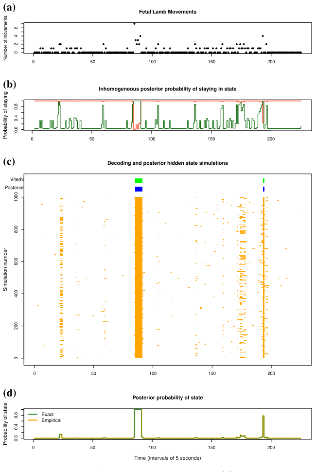
Summary. The paper addresses two tasks for hidden Markov models: computing exact posterior distributions of summary statistics of the hidden state sequence via finite Markov chain imbedding (FMCI), and improving decoding through hybrid decoding with a proposed tuning-parameter rule called the Artemis analysis. The authors prove Theorem 1, that the hidden state sequence conditional on the observed sequence is an inhomogeneous first-order Markov chain, and they use it to build FMCI transition matrices for the number of jumps, number of positions in a state, exact run lengths, and longest run. These FMCI results are validated against 1000 posterior samples on the fetal lamb movement data. For decoding, the paper rederives the hybrid risk as a weighted geometric mean, introduces the Artemis plot for choosing the tuning parameter alpha, and reports simulation results suggesting that hybrid decoding improves block-wise accuracy relative to Viterbi and posterior decoding for intermediate block sizes. Code is provided in a GitHub repository.
Significance. The FMCI part is sound and clearly connected to Theorem 1: the theorem is standard and the proof is correct, and the comparison with posterior samples is an appropriate internal consistency check rather than circular reasoning. The alternative weighted-geometric-mean derivation of hybrid decoding is clean and complements the existing decision-theoretic framework. The provision of reproducible code is a genuine strength. The main novel methodological contribution, however, is the Artemis rule for selecting alpha, and the current evidence for the central decoding claim rests on only ten simulations per setting, with tuning and evaluation performed on the same simulated data and no error bars. If the decoding claim can be supported by a more rigorous evaluation, the paper will be a useful methods contribution for practitioners; as it stands, the decoding part is not yet convincing enough to support the abstract's claim of increased performance.
major comments (4)
- [Section 4.4, Figures 13-14] The evaluation of hybrid decoding is in-sample. Section 4.4 states that "The alpha's used for hybrid are the optimal alpha's found using the Artemis plots in Figure 10," and those optimal alpha values were determined in Section 4.2 from the same 10 simulated (x,y) pairs per setting that are subsequently used to compute block-wise accuracy. This protocol allows selection bias to inflate the reported gains, which are often modest (ratios from roughly 1.01 to 1.48 relative to Posterior decoding). With only 10 replicates and no error bars, the observed improvement could be within simulation noise. An out-of-sample or cross-validated evaluation, together with uncertainty estimates, is required before the abstract claim that "hybrid decoding shows increased performance" can be considered established.
- [Section 4.2, Figure 10] The 45-degree rule for choosing alpha is not well-defined as stated. The axes are "scaled using the minimum and maximum value for each axis," independently for each simulation. The angle of the tangent to the bow-shaped curve is therefore not invariant under affine rescaling of the axes, and the reported optimal alpha could change simply by changing the plotting range. The authors need to either define alpha selection by an explicit criterion that does not depend on plotting scale, such as a point on a Pareto frontier defined by a meaningful trade-off, or demonstrate that the 45-degree rule is robust to reasonable changes in axis scaling. As written, the Artemis rule is an arbitrary heuristic rather than a principled estimator.
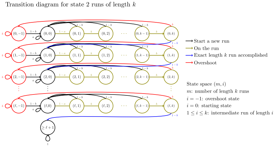
- [Sections 3.2.1-3.2.4] The matrix displays for the FMCI transition matrices are incomplete and cannot be independently verified from the printed text. For example, in Section 3.2.1 the block B(a,b) is defined but the displayed matrix Lambda does not fill in the entries of the block structure explicitly; in Section 3.2.3 the row "1-b 0 b" leaves the first-column entry unspecified. Since these transition matrices are the core of the FMCI distributional claims, the authors should provide complete, unambiguous matrix definitions, either as displayed matrices or by explicit equation numbers, and should check that the rendering is not garbled.
- [Section 3.2.1 and Section 5] The FMCI distributions are exact only conditional on the user-chosen truncation level ell. The last entry of the imbedding vector lumps all counts exceeding ell into one absorbing state, as stated in Section 3.2.1. This is a real limitation, and the manuscript should report the tail probability or a sensitivity analysis for the choice of ell, particularly for the longest-run distribution where the tail is of direct interest. The current text acknowledges the truncation but does not quantify its impact on the reported posterior distributions.
minor comments (5)
- [Section 3.2.1] There is a typo: "we that have Lambda = Lambda(a,b)" should read "we have Lambda = Lambda(a,b)".
- [Equation (4)] In the denominator of the conditional initial state probability, the notation "Phi(x1|y1=i)" should be "Phi(x1|i)" for consistency with the rest of the paper.
- [Section 3.2.2] The block matrix B(a,b) for the number of positions appears to have the first row as (1-b, a) and the second as (a, 1-a), but the accompanying text and Figure 7 should clarify which entries correspond to transitions that increment the count; currently the notation is confusing.
- [Section 4.4, Figure 13 caption] The phrase "blocks of size two any two pairs in the sequence" is unclear and should be reworded to "blocks of size two consist of any two consecutive positions in the sequence."
- [Section 2.2] There is a typo: "probablity" should be "probability" in the description of the conditional probability used in the Artemis plot.
Circularity Check
Hybrid decoding gains are measured on the same simulations used to tune α; the FMCI part is self-contained.
-
fitted input called prediction
[Section 4.2 and Section 4.4, Figure 10 and Figure 13 captions]
"In Figure 10 we have used 10 simulations for each of the three cases ... The optimal α is the average of the 10 simulations for each case. ... The αs used for hybrid are the optimal αs found using the Artemis plots in Figure 10."
The tuning parameter α is selected from exactly the same simulated (x,y) pairs that are then used to report hybrid block-wise accuracy (Figure 13: 'based on 10 simulations for each block size'). No held-out or independently generated sequences are used for evaluation, so the reported hybrid gains are in-sample fits rather than out-of-sample predictions. The central claim that 'hybrid decoding shows increased performance' is therefore partly forced by the tuning procedure itself, and the 45-degree Artemis rule is never tested on data that did not contribute to choosing α.
full rationale
The FMCI component is not circular: Theorem 1 is proved in the paper, and the posterior distributions for jumps, state occupancy, exact run lengths, and longest run follow by exact finite products of the inhomogeneous transition matrices. The agreement between FMCI and empirical simulation in Figure 2 is an internal consistency check, not a circular derivation. The weighted-geometric-mean derivation of the hybrid loss is an algebraic identity and is also not circular. The only substantive circularity is in the hybrid decoding demonstration: the same 10 simulated sequences are used both to select the optimal α via the Artemis plot and to measure the block-wise accuracy that supports the abstract's claim of increased performance. This is an in-sample evaluation with no cross-validation or external benchmark, so the reported improvement is not an independent prediction. The arbitrary min-max scaling and 45-degree tangent heuristic are correctness risks rather than circularity per se, but they compound the in-sample nature of the validation. Score 6 reflects that the central decoding claim is partially reduced to a fitted-input evaluation, while the FMCI half of the paper remains independent and self-contained.
Assumptions & free parameters
free parameters (5)
- HMM parameters for fetal movement data =
pi=(1,0); Gamma=[[0.989,0.011],[0.287,0.703]]; lambda=(0.278,3.217)
- HMM parameters for earthquakes data =
pi=(1,0); Gamma=[[0.928,0.072],[0.119,0.881]]; lambda=(15.4,26.0)
- Simulation difficulty parameters a and q =
a in {10,5,2}; q in {0.8,0.5,0.1}
- FMCI truncation level L =
L=7 for fetal data jumps (similar per statistic)
- Artemis simulation length n =
n=10^5
assumptions (5)
- domain assumption The observed sequence comes from a first-order hidden Markov model with fixed or MLE-estimated parameters.
- standard math The hidden state sequence conditional on observations is an inhomogeneous first-order Markov chain (Theorem 1).
- domain assumption The four summary statistics admit finite Markov chain imbedding with a chosen truncation level L.
- ad hoc to paper The Artemis plot's 45-degree tangent rule selects a good tuning parameter alpha for hybrid decoding.
- domain assumption Simulations from the fitted HMM are representative of the real data for choosing alpha.
Cite this review
Pith. "Pith review of Advanced posterior analyses of hidden Markov models: finite Markov chain imbedding and hybrid decoding." pith.science (2026). https://pith.science/paper/3RRIYOI4
@misc{pith2026250415156,
  author       = {Pith},
  title        = {Pith review of: Advanced posterior analyses of hidden Markov models: finite Markov chain imbedding and hybrid decoding},
  year         = {2026},
  howpublished = {\url{https://pith.science/paper/3RRIYOI4}},
  note         = {Machine review of arXiv:2504.15156}
}
read the original abstract
Two major tasks in applications of hidden Markov models are to (i) compute distributions of summary statistics of the hidden state sequence, and (ii) decode the hidden state sequence. We describe finite Markov chain imbedding (FMCI) and hybrid decoding to solve each of these two tasks. In the first part of our paper we use FMCI to compute posterior distributions of summary statistics such as the number of visits to a hidden state, the total time spent in a hidden state, the dwell time in a hidden state, and the longest run length. We use simulations from the hidden state sequence, conditional on the observed sequence, to establish the FMCI framework. In the second part of our paper we apply hybrid segmentation for improved decoding of a HMM. We demonstrate that hybrid decoding shows increased performance compared to Viterbi or Posterior decoding (often also referred to as global or local decoding), and we introduce a novel procedure for choosing the tuning parameter in the hybrid procedure. Furthermore, we provide an alternative derivation of the hybrid loss function based on weighted geometric means. We demonstrate and apply FMCI and hybrid decoding on various classical data sets, and supply accompanying code for reproducibility.
Figures


Figures from the paper (11 more)




Forward citations
Cited by 1 Pith paper
-
Branch-and-bound method for calculating Viterbi path in triplet Markov models
A branch-and-bound algorithm with multiple bound types computes the most probable marginal path in triplet Markov models much faster than exhaustive search, with m-Viterbi giving the best lower bounds.
Reference graph
Works this paper leans on
-
[1]
Aston, J. A. D. and Martin, D. E. K. (2007). Distributions associated with general runs and patterns in hidden Markov models . The Annals of Applied Statistics , 1(2):585 -- 611
work page 2007
-
[2]
Burge, C. and Karlin, S. (1997). Prediction of complete gene structures in human genomic DNA . Journal of molecular biology , 268(1):78--94
work page 1997
-
[3]
Coll Macià, M., Skov, L., Bæk, Z. E. D., and Hobolth, A. (2025). Enhancement of hidden M arkov model analyses for improved inference of archaic introgression in modern humans. Available on bioRxiv
work page 2025
-
[4]
R., Krogh, A., and Mitchison, G
Durbin, R., Eddy, S. R., Krogh, A., and Mitchison, G. (1998). Biological sequence analysis: probabilistic models of proteins and nucleic acids . Cambridge university press
work page 1998
-
[5]
Dutheil, J. Y. (2017). Hidden M arkov models in population genomics. In Hidden Markov models: Methods and protocols , pages 149--164. Springer
work page 2017
-
[6]
Fu, J. C. and Koutras, M. V. (1994). Distribution theory of runs: A M arkov chain approach. Journal of the American Statistical Association , 89(427):1050--1058
work page 1994
-
[7]
Guttorp, P. (2018). Stochastic modeling of scientific data . Chapman and Hall/CRC
work page 2018
-
[8]
Hobolth, A. and Jensen, J. L. (2005). Applications of hidden M arkov models for characterization of homologous DNA sequences with a common gene. Journal of Computational Biology , 12(2):186--203
work page 2005
Show all 17 references
-
[9]
and Lember, J
Kuljus, K. and Lember, J. (2023). Pairwise M arkov models and hybrid segmentation approach. Methodology and Computing in Applied Probability , pages 25 (2), 67
2023
-
[10]
and Koloydenko, A
Lember, J. and Koloydenko, A. A. (2014). Bridging V iterbi and P osterior decoding: A generalized risk approach to hidden path inference based on hidden M arkov models. Journal of Machine Learning Research , 15(1):1--58
2014
-
[11]
Leroux, B. G. and Puterman, M. L. (1992). Maximum-penalized-likelihood estimation for independent and M arkov-dependent mixture models. Biometrics , 48(2):545--558
1992
-
[12]
Lindgren, G. (1978). Markov regime models for mixed distributions and switching regressions. Scandinavian Journal of Statistics , 5(2):81--91
1978
-
[13]
Martin, D. E. (2020). Distributions of pattern statistics in sparse M arkov models. Annals of the Institute of Statistical Mathematics , 72:895--913
2020
-
[14]
Skov, L., Hui, R., Shchur, V., Hobolth, A., Scally, A., and Schierup, M. (2018). Detecting archaic introgression using an unadmixed outgroup. PLOS Genetics , 14:e1007641
2018
-
[15]
Turner, R. (2008). Direct maximization of the likelihood of a hidden M arkov model. Computational Statistics & Data Analysis , 52(9):4147--4160
2008
-
[16]
and Holmes, C
Yau, C. and Holmes, C. C. (2013). A decision-theoretic approach for segmental classification. The Annals of Applied Statistics , pages 1814--1835
2013
-
[17]
L., and Langrock, R
Zucchini, W., MacDonald, I. L., and Langrock, R. (2016). Hidden M arkov Models for Time Series: An Introduction Using R . CRC Press, 2 edition
2016
Reviewed August 16, 2026 · model on record in the stance chip above.
Discussion (0). Continue with ORCID to comment.