REVIEW 4 major objections 5 minor 13 references
AI Alignment in Medical Imaging: Unveiling Hidden Biases Through Counterfactual Analysis
T0 review · 4 major / 5 minor · reviewed 2026-08-16 · deepseek-v4-flash
Pith's one-line read A statistical test using generated counterfactual X-rays can reveal whether medical AI models are biased by sensitive attributes like race.
desk verdict The central algorithm's t-statistic is invalid as written, so the reported p-values and the claimed alignment with ECA do not hold up; still, the paper tackles a real problem and deserves a serious referee with an invitation to fix the statistics and break the circular validation. read the letter →
The pith
A machine-rendered reading of the paper's core claim, the machinery that carries it, and where it could break.
The reading
What carries the argument
The load-bearing identity is Theorem 4.2: given a latent representation $Z$ that is a valid adjustment set, a classifier is counterfactually invariant iff $\mathbb{E}[\hat Y g(A,Z)] = \mathbb{E}[\hat Y h(Z)]$, which follows from a law-of-total-variance argument. The machinery that turns this identity into a test is a conditional latent diffusion model with a disentangling transform $\phi_{\lambda,\delta}$ that makes the representation approximately independent of the attribute $A$ (trained by minimizing a mutual-information lower bound), used to generate counterfactual images; the test statistic is a paired $t$-test comparing the two expectations estimated on separately split datasets.
What would settle it
Construct a synthetic structural causal model where the latent representation deliberately omits a disease-relevant confounder, train classifiers with known counterfactual bias, and check whether CIT-LR still tracks the true expected counterfactual accuracy; if the test's p-values stop correlating with ground truth when the adjustment set is incomplete, the key assumption is thereby refuted.
Extended reading notes
Core claim
The paper's central claim is that a model's counterfactual invariance with respect to a sensitive attribute can be tested from observed samples by checking the identity $\mathbb{E}[\hat Y g(A,Z)] = \mathbb{E}[\hat Y h(Z)]$, where $Z$ is a latent representation, $g(a,z) = \mathbb{E}[\hat Y \mid A=a, Z=z]$ and $h(z) = \mathbb{E}[\hat Y \mid Z=z]$. Under the conditional ignorability assumption that $Z$ is a valid adjustment set, this identity holds exactly when the classifier is counterfactually invariant. The proposed CIT-LR algorithm implements the test by training a disentangled conditional latent diffusion model to generate counterfactual images with the sensitive attribute changed, estimating $g$ and $h$ from those generations, and running a two-sample Student's $t$-test on $\hat Y g(A,Z)$ versus $\hat Y h(Z)$. The authors report that in experiments on synthetic data and on cheXpert and MIMIC-CXR, CIT-LR rejects the null hypothesis when the expected counterfactual accuracy is low and fails to reject when it is high, providing stronger consistency than demographic parity and equality of opportunity.
Load-bearing premise
The test collapses if the latent representation learned by the generative model does not capture every factor that matters for the diagnosis, because then the statistical equality used to judge invariance is not guaranteed to hold.
Editorial extensions
If this is right
- Pretrained diagnostic classifiers can be audited for sensitive-attribute bias without collecting any counterfactual images, using only the training data and a generative model.
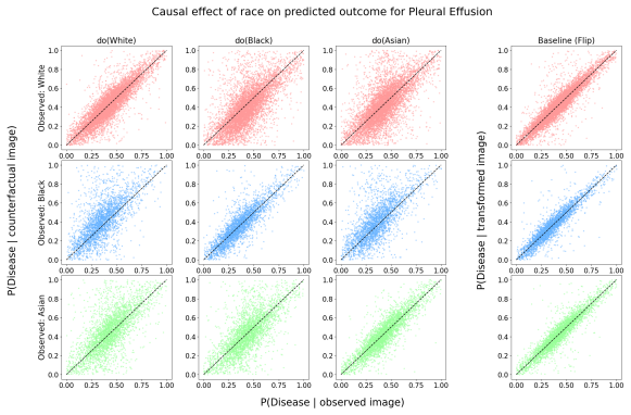
- The test splits diseases into those where near-invariant classifiers exist (consolidation) and those where most classifiers are non-invariant (cardiomegaly, edema, pleural effusion), giving a concrete target for fairness improvement.
- Because it is a hypothesis test with p-values, the method provides a significance threshold for model selection or regulatory compliance rather than a point estimate.
- On the tested datasets, demographic parity and equality of opportunity both flag invariant models as biased and miss biased ones; CIT-LR is claimed to be more consistent, so replacing association-based audits with a counterfactual test could change which models get deployed.
Reading between the lines
- If the latent representation captures all disease-relevant factors, the same machinery could audit other sensitive attributes (age, sex) and other medical modalities, not just chest X-rays.
- The test's validity could be checked by a 'negative control' experiment: train classifiers with deliberately injected known confounding, ablate the disease-relevant latent factor, and see whether CIT-LR's verdict flips; if it does not, the causal assumption is doing the work.
- The disentangling transform $\phi$ is optimized via a mutual-information lower bound; since lower bounds can be loose, the actual degree of disentanglement could be reported as a diagnostic of the test's reliability.
- A practitioner might use CIT-LR not only to reject bad checkpoints but also to rank checkpoints of the same architecture, choosing the one whose p-value indicates invariance, before clinical deployment.
Signed reviews
Editorial analysis
A structured set of objections, weighed in public.
Referee Report
Summary. The paper proposes CIT-LR, a statistical test for counterfactual invariance (CI) of a pretrained medical imaging classifier with respect to a sensitive attribute A. The test combines a conditional latent diffusion model (CLDM) with a disentangling transformation to learn the functions g(a,z)=E[Y|A=a,Z=z] and h(z)=E[Y|Z=z], then uses a t-test on E[Y g(A,Z)] versus E[Y h(Z)] to decide CI. Experiments on synthetic data, cheXpert, and MIMIC-CXR compare CIT-LR p-values with an Expected Counterfactual Accuracy (ECA) ground truth and with DP/EO baselines, claiming stronger alignment. As written, however, the central statistical step is invalid and the validation is partly circular.
Significance. The intended contribution—a practical, falsifiable statistical audit for demographic bias in diagnostic models—is important and timely. If the test were valid, it would improve on association-based fairness metrics by targeting counterfactual invariance. The paper also makes useful practical steps: it provides code, considers 100 classifiers per dataset, and reports comparisons with DP/EO. However, the significance is currently not realized: the t-statistic in Algorithm 1 is mathematically incorrect, the quantities computed in Step 2 do not match the functions learned in Step 1, and the real-world ECA ground truth is derived from the same unproved adjustment-set assumption that the test uses. These issues undermine the central empirical claim.
major comments (4)
- [Section 5, Algorithm 1, Step 3 (line 16)] The t-statistic t = sqrt(|Dtest|)(mu_Z - mu_AZ)/(sigma_Z - sigma_AZ) with |Dtest|-1 degrees of freedom is not a valid test statistic for any standard hypothesis test. The denominator is the difference of two estimated standard deviations, not a standard error of the difference of means; it can be zero or negative, making the statistic unstable and uninterpretable. The surrounding text says a paired t-test is used, while the algorithm says a two-sample Student's t-test; neither would have this form. Since every p-value reported in Figures 2-4 and Tables 12-13 is computed from this invalid statistic, the central empirical claim that CIT-LR 'rejects when ECA is low and does not when the ECA is high' is unsupported as written.
- [Section 5, Algorithm 1, Steps 1-2] There is a mismatch between the functions learned in Step 1 and the inputs on which they are evaluated in Step 2. Step 1 defines ghat(a,z) and hhat(z) using zhat_0 ~ p_theta(zhat_0 | z,a), i.e., reverse-diffusion samples from the CLDM. Step 2, however, computes ghat(a, ztilde_T) and hhat(ztilde_T) with ztilde_T ~ q_theta(ztilde_T | ztilde_0), i.e., forward-diffusion noised latents. These are different random variables, so the test is not actually evaluating E[Y|A=a,Z=z] or E[Y|Z=z] at the representation used in Theorem 4.2. The estimated quantities therefore do not correspond to the null hypothesis of the test.
- [Section 6.3 and Appendix E] The real-world ECA ground truth is not independent confirmation of the method. In Section 6.3 and Appendix E, ECA is computed using the equality E[Y|do(A=a),Z=z] = E[Y|A=a,Z=z] from Lemma D.3, with Z being the learned CLDM latent representation. The test's null hypothesis in Theorem 4.2 relies on exactly the same equality and the same Z. Hence the alignment between CIT-LR p-values and ECA on cheXpert and MIMIC-CXR is partly by construction and does not provide independent evidence that the test detects true counterfactual invariance. The paper's Impact Statement concedes that the key assumption that latent representations capture all relevant factors 'is not adequately proved.'
- [Section 3.3, Eq. (3)] The disentanglement condition Z perpendicular A is not established. The optimization minimizes a lower bound on the mutual information I(phi(z0), a) using the MINE estimator, not the true mutual information, and no theorem guarantees that the resulting representation satisfies the valid-adjustment-set condition required by Theorem 4.2 and Lemma D.3. This is a load-bearing gap in the identification argument, since the validity of the entire test depends on this assumption.
minor comments (5)
- [Section 5] The terminology is inconsistent: the text says a paired t-test is used, while Algorithm 1 Step 3 says a two-sample Student's t-test. The paper should state one correct test and use it consistently.
- [Throughout] There are numerous typos and formatting issues, including 'spECAfic' in place of 'specific', 'ff.' in place of 'if and only if', 'DECAsionTreeClassifier' in Table 1, and 'Equality of Opportunity' versus 'Equal Opportunity' in Section 6.1.
- [Figures 2-4] The figures plot log-transformed p-values, but the handling of p-values that are exactly zero or near machine precision is not described; clarify the transformation used.
- [References] The reference list contains several duplicate entries (e.g., Dhariwal and Nichol 2021a/2021b, Müller-Franzes et al. 2023a/2023b) and some incomplete entries; please consolidate and complete the bibliography.
- [Section 6.1] The baseline tests for DP and EO are described as paired t-tests, but the exact test statistic and degrees of freedom are not specified, making the comparison with CIT-LR difficult to assess even setting aside the invalid statistic in Algorithm 1.
Circularity Check
Real-world validation of CIT-LR against ECA is partially circular: the ECA ground truth is computed from the same learned latent representation and the same conditional-ignorability equality that defines the test's null hypothesis.
-
self definitional
[Section 6.3 (Performance Evaluation Metric); Theorem 4.2 proof and Appendix E]
"In this case, we can compute the ECA since it holds E[ ˆY |do(A = a), Z = z] = E[ ˆY |A = a, Z = z]. We refer the reader to App. E for a proof of this claim."
The test's null hypothesis is E[Y g(A,Z)] = E[Y h(Z)] with g=E[Y|A,Z], h=E[Y|Z]; Theorem 4.2's proof reduces counterfactual invariance to this equality using 'the conditional ignorability assumption' E[Y|do(A=a),Z=z]=E[Y|A=a,Z=z]. The real-world ECA is then computed from that same equality and the same learned CLDM representation Z (Appendix E). Thus the claimed agreement between CIT-LR p-values and ECA on cheXpert/MIMIC-CXR is a consistency check of the method's own unproved representation assumption, not an independent confirmation. The Impact Statement concedes: 'our method relies on the key assumption that the latent representations capture all the relevant factors, which is not adequately proved.'
full rationale
The abstract identification result in Theorem 4.2 is not itself circular: it is a self-contained law-of-total-variance characterization of counterfactual invariance, and the synthetic experiments use known DGPs that provide some independent evidence. However, the real-world evaluation is partially circular. The ECA ground truth is not measured externally; it is computed using the same learned CLDM latent Z and the same conditional-ignorability equality E[Y|do(A=a),Z=z]=E[Y|A=a,Z=z] that the test's null hypothesis relies on. Therefore the paper's central real-data claim—that CIT-LR 'rejects the hypothesis test when ECA is low and does not when the ECA is high'—is largely a comparison of two quantities derived from the same assumption. The paper itself flags the load-bearing assumption as not adequately proved. Separately, Algorithm 1's t-statistic t = sqrt(|Dtest|)(mu_Z - mu_AZ)/(sigma_Z - sigma_AZ) is not a valid two-sample Student's t-statistic (the denominator is a difference of standard deviations, not a standard error); this is a correctness defect rather than a circularity, but it further undermines the reported p-values as written. Overall score 6 reflects partial circularity: the synthetic validation and the theoretical equivalence are independent content, but the real-world validation reduces substantially to the model's own assumptions.
Assumptions & free parameters
free parameters (3)
- lambda (perturbation scale in phi) =
1e-3
- diffusion noise scale and steps =
beta scaled to 20%, T=250
- Monte Carlo sample count n for g and h =
not reported
assumptions (4)
- ad hoc to paper Z is a valid adjustment set for {A, Y} in the CLDM causal graph.
- domain assumption Conditional ignorability: E[Y|do(A=a),Z=z] = E[Y|A=a,Z=z].
- ad hoc to paper The disentangled representation satisfies Z perpendicular A.
- domain assumption The CLDM faithfully realizes the intervention do(A=a) while preserving disease features.
Cite this review
Pith. "Pith review of AI Alignment in Medical Imaging: Unveiling Hidden Biases Through Counterfactual Analysis." pith.science (2026). https://pith.science/paper/LHDQC4AI
@misc{pith2026250419621,
  author       = {Pith},
  title        = {Pith review of: AI Alignment in Medical Imaging: Unveiling Hidden Biases Through Counterfactual Analysis},
  year         = {2026},
  howpublished = {\url{https://pith.science/paper/LHDQC4AI}},
  note         = {Machine review of arXiv:2504.19621}
}
read the original abstract
Machine learning (ML) systems for medical imaging have demonstrated remarkable diagnostic capabilities, but their susceptibility to biases poses significant risks, since biases may negatively impact generalization performance. In this paper, we introduce a novel statistical framework to evaluate the dependency of medical imaging ML models on sensitive attributes, such as demographics. Our method leverages the concept of counterfactual invariance, measuring the extent to which a model's predictions remain unchanged under hypothetical changes to sensitive attributes. We present a practical algorithm that combines conditional latent diffusion models with statistical hypothesis testing to identify and quantify such biases without requiring direct access to counterfactual data. Through experiments on synthetic datasets and large-scale real-world medical imaging datasets, including \textsc{cheXpert} and MIMIC-CXR, we demonstrate that our approach aligns closely with counterfactual fairness principles and outperforms standard baselines. This work provides a robust tool to ensure that ML diagnostic systems generalize well, e.g., across demographic groups, offering a critical step towards AI safety in healthcare. Code: https://github.com/Neferpitou3871/AI-Alignment-Medical-Imaging.
Figures


Figures from the paper (11 more)




Reference graph
Works this paper leans on
-
[1]
A., R. L. M., Echeveste, R., and Ferrante, E. (2022). Addressing fairness in artificial intelligence for medical imaging.Nature Communications, 13(1):4581. Adamson, A. and Smith, A. (2018). Machine learning and health care disparities in dermatology. JAMA Dermatology, 154(11):1247–1248. Austin, J., Johnson, D. D., Ho, J., Tarlow, D., and van den Berg, R. ...
work page 2022
-
[4]
Same setting is applied to Chexpert and MIMIC-CXR dataset
hidden_layer_sizes=(16, 4), activation=’relu’, solver=’adam’, max_iter=500 Table 1: Machine learning models and their hyperparameters used for classification on the synthetic datasets G.2 Base Classifiers for cheXpert and MIMIC-CXR Model architectures. Same setting is applied to Chexpert and MIMIC-CXR dataset. The diagnosis models, namely the disease clas...
work page 2016
-
[5]
Hence, the claim follows by Lemma D.2
In this graph, the variableZ is a valid adjustment set for{A, ˆY}. Hence, the claim follows by Lemma D.2. We can now prove Theorem 4.2. Proof of Theorem 4.2.First of all, note that by the conditional ignorability assumption we have that E[ ˆY |do(A =a), Z = z] = E[ ˆY |A =a, Z = z] for alla. Hence, a modelf(X) is counterfactually invariant with respect to...
work page 1991
-
[6]
Johnson, A. E. W., Pollard, T. J., Greenbaum, N. R., Lungren, M. P., ying Deng, C., Peng, Y., Lu, Z., Mark, R. G., Berkowitz, S. J., and Horng, S. (2019b). Mimic-cxr-jpg, a large publicly available database of labeled chest radiographs. Jülich Supercomputing Centre (2021). JUWELS Cluster and Booster: Exascale Pathfinder with Modular Supercomputing Archite...
work page 2019
-
[7]
D Proof of Theorem 4.2 In order to prove Theorem 4.2, we use the well-known concept of valid adjustment set in causal inference. For a review on this notion and its properties we refer the reader to , e.g., Pearl [2009], Peters et al. [2017]. Definition D.1(Valid Adjustment Set). LetG be a causal graph and letA, ˆY be disjoint (sets of) nodes inG. A set o...
work page 2009
-
[9]
male”, and55.5% patients labeled as “female
and bY∼N (0, 1). • log-exponent: fY (Zn) = log(exp(ωY·Zn) +bY ), withωY∼N (0,I ) and bY∼N (5, 1). • sin: fY (Zn) =ωY· sin(Zn) +bY, withωY∼N (0,I ) and bY∼N (2, 1). Here, ωY and bY are fixed model parameters during the generation process. During the simulation, we take the following values on the hyperparametersT = 3,k = 32,σ = 0.01. The SCM’s parameterMt,...
work page 2019
-
[10]
25.10 27.22 CLDM 22.14 26.10 DLDM 21.79 25.89 I.1 Evaluate CI of diagnosis models The goal of this set of experiments is to better understand to which extent the racial attributes influence the predictions of a given diagnostic model. We choose the Densenet121 classifier [Huang et al., 2016] from our diagnosis model pool as an example. For this model, we ...
work page 2016
-
[12]
In this section, we use the acronym DLDM (Disentangled Latent Diffusion Model) to denote a CLDM with disentangled representations. Evaluation Metrics.We consider two evaluation metrics: • (FID score) The Fréchet Inception Distance (FID) evaluates the statistical similarity of extracted features from two sets of images. Hence it can be used to measure the ...
work page 2021
Show all 13 references
-
[29]
He, K., Zhang, X., Ren, S., and Sun, J. (2015). Deep residual learning for image recognition. Higgins, I., Matthey, L., Pal, A., Burgess, C. P., Glorot, X., Botvinick, M. M., Mohamed, S., and Lerchner, A. (2017). beta-vae: Learning basic visual concepts with a constrained vari...
2015 arXiv
-
[30]
forensics
Kusner, M. J., Loftus, J. R., Russell, C., and Silva, R. (2017b). Counterfactual fairness. In Advances in Neural Information Processing Systems 30: Annual Conference on Neural Information Processing Systems 2017, December 4-9, 2017, Long Beach, CA, USA, pages 4066–4076. Montei...
2017 arXiv
-
[2015]
and inception-V3Szegedy et al. [2015]. For each type of backbone we select multiple variations. For Densenet, we select Densenet 121, Densenet 169 and Densenet
2015
-
[2024]
with Def. 4.1. Almost Sure CI (a.s.-CI):Almost Sure CI (a.s.-CI), as defined by Fawkes et al. [2022a], requires that a variableY remains exactly the same almost surely under any interventions on A. Formally,Y satisfies a.s.-CI with respect toA if it holdsY |do(A =a) =Y |do(A =...
2021
-
[2915]
Bordes, F., Balestriero, R., and Vincent, P. (2022). High fidelity visualization of what your self-supervised representation knows about.Transactions on Machine Learning Research. Chernozhukov, V., Newey, W., Quintas-Martinez, V., and Syrgkanis, V. (2022). Riesznet and forestr...
2022 arXiv
Reviewed August 16, 2026 · model on record in the stance chip above.
Discussion (0). Continue with ORCID to comment.