Learning Laplacian Positional Encodings for Heterophilous Graphs

Danai Koutra; Dexiong Chen; Jenna Wiens; Jiong Zhu; Michael Ito

REVIEW 3 major objections 4 minor 14 references

Learning Laplacian Positional Encodings for Heterophilous Graphs

T0 review · 3 major / 4 minor · reviewed 2026-08-16 · deepseek-v4-flash

Challenge this review Re-run · record.json Download PDF Read on arXiv ↗ Review JSON

Pith's one-line read Learnable Laplacian encodings that weight the full spectrum recover a general class of spectral graph distances and improve node classification on heterophilous graphs by up to 35% on synthetic and 14% on real-world benchmarks.

desk verdict The expressivity proof covers d=n while the deployed LLPE uses d=128, but the heterophily result and the broad empirical evaluation are solid enough to deserve a proper review. read the letter →

arxiv 2504.20430 v1 pith:W4KW2IA6 submitted 2025-04-29 cs.LG

Michael Ito , Jiong Zhu , Dexiong Chen , Danai Koutra , Jenna Wiens This is my paper · ORCID

classification cs.LG

keywords graphneuralnetworkspositionalencodingsheterophilyLaplacianChebyshevpolynomialsspectraltheorynodeclassificationtransformers

verification ladder T0 review T1 audit T2 compute T3 formal

The pith

A machine-rendered reading of the paper's core claim, the machinery that carries it, and where it could break.

The reading

This paper claims that standard graph positional encodings, especially Laplacian encodings built from the first few eigenvectors, miss the structure that matters on heterophilous graphs, where connected nodes tend to have different labels. To fix this, it introduces Learnable Laplacian Positional Encodings (LLPE), which weight all eigenvectors of the graph Laplacian through a learned function of the eigenvalues. The paper proves that LLPE can approximate a broad class of spectral graph distances, encompassing commute time, diffusion distance, and biharmonic distance, and that its generalization error is controlled by the norm of the learned coefficients. Across twelve benchmarks and several GNN backbones, LLPE improves node classification accuracy by up to 35% on synthetic graphs and up to 14% on real-world graphs, with the largest gains on heterophilous benchmarks and on nodes in locally heterophilous regions of globally homophilous graphs.

What carries the argument

The load-bearing object is the learned spectral weighting function $h(\lambda; \theta) = \sum_{m=0}^{M} \theta_m T_m(\tilde{\lambda})$, a truncated Chebyshev series evaluated at normalized Laplacian eigenvalues. Applied as $W_{\mathrm{LLPE}}$ with entries $h(\lambda_i; \theta_j)$, it converts the full eigenvector matrix $U$ into a positional encoding whose per-node Euclidean distances approximate a target spectral distance. The mechanism carries the argument because the Chebyshev weights are smooth universal approximators on the spectrum, so the same encoding can act as a low-pass filter on homophilous graphs and a high-pass filter on heterophilous ones; the smoothness of the weights also keeps the hypothesis class low-dimensional, which the paper shows yields favorable Rademacher complexity.

What would settle it

Train LLPE with $d=128$ on a heterophilous graph where the class structure is known to live in a specific high-frequency eigenspace, then compare its node classification accuracy to that of a PE built directly from the exact label-correlated eigenvectors. A systematically large gap would falsify the practical expressivity claim, since the theory does not guarantee that the fixed-dimensional Chebyshev encoding can recover that subspace.

Watch

Extended reading notes

Core claim

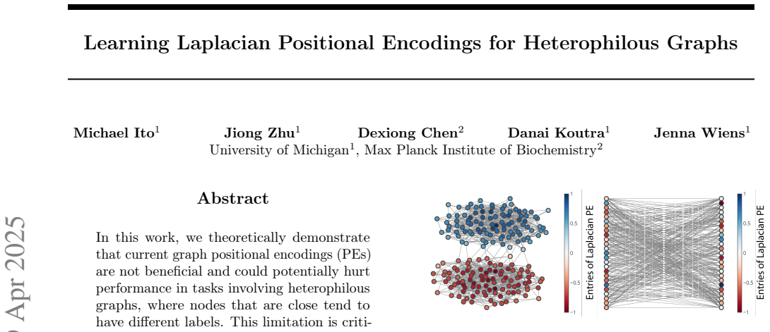
The central claim is that the eigenvectors of the graph Laplacian that carry the label-relevant structure shift with the homophily of the graph: in homophilous stochastic block models the first nontrivial eigenvectors encode communities, while in heterophilous block models it is the last eigenvectors that do so, and the first ones provably fail. Consequently, any positional encoding fixed to the low end of the spectrum cannot serve both regimes. LLPE removes this restriction by forming $P_{\mathrm{LLPE}} = U W_{\mathrm{LLPE}}$, where the columns of $W_{\mathrm{LLPE}}$ are truncated Chebyshev series evaluated at the eigenvalues, so the network learns which spectral directions matter for the task. The paper proves (Theorem 4.3) that, with output dimension equal to $n$, LLPE can recover any distance of the form $f_r(i,j)^2 = \sum_k r(\lambda_k)(u_k[i] - u_k[j])^2$ for a nonnegative weight function $r$, thereby subsuming several known graph distances and capturing both low- and high-frequency structure. It also proves Rademacher-complexity bounds showing that the Chebyshev-coefficient norm, not the series order, controls generalization.

Load-bearing premise

The proof that LLPE can approximate any spectral distance assumes the output dimension equals the number of nodes, while the deployed version fixes a much smaller output dimension, and the paper gives no theorem that the reduced encoding still achieves the same approximation.

Editorial extensions

If this is right

LLPE can be added to any GNN or graph transformer without changing the model, improving accuracy on heterophilous benchmarks and on locally heterophilous regions of homophilous graphs.
Because LLPE provably approximates commute time, diffusion distance, and biharmonic distance, a single learned encoding can replace several purpose-built positional encodings.
The generalization bound implies that increasing the Chebyshev order $M$ improves expressivity without degrading generalization, as long as the learned coefficient norm stays small.
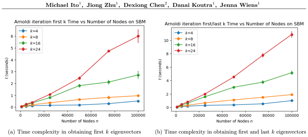
For large graphs, the approximate LLPE using only the first and last $k$ eigenvectors obtained by Arnoldi iteration preserves most of the benefit while keeping computation feasible.
Existing learnable PEs that process the full eigenvector matrix with MLPs or transformers scale poorly in the node count; LLPE's parameter count depends on $M$, not $n$, so it scales more gracefully.

Reading between the lines

Editorial extensions of the paper, not claims the author makes directly.

The expressivity theorem is proven with output dimension $d = n$ using narrow Gaussian bumps approximated by Chebyshev series; the practical LLPE fixes $d = 128$, so whether the fixed-dimensional encoding retains the full approximation power on real graphs is an empirical premise rather than a proven guarantee.
LLPE's learned weight curve $h(\lambda)$ could be inspected post-hoc to identify which spectral bands actually mediate the label structure of a dataset, offering a diagnostic for heterophily that is not currently part of the paper.
The method's ability to capture both same-label and opposite-label proximity suggests it could transfer to link prediction or graph-level tasks in heterophilous settings, though the paper only evaluates node classification.
One could test LLPE against a directly supervised selection of eigenvectors (e.g., chosen by label correlation) on heterophilous benchmarks; a large gap would indicate that the Chebyshev parametrization, rather than spectral content, is the bottleneck.

Share X Bluesky LinkedIn Reddit HN

Signed reviews

No signed human review yet.

Editorial analysis

A structured set of objections, weighed in public.

Desk editor's note, referee report, and a circularity audit.

Desk Editor's Note

read the letter

Colleague—

This one is worth a serious look. The crispest new piece is Theorem 3.2: in a heterophilous SBM the last k−1 Laplacian eigenvectors recover the communities while the first k do not. It gives a principled reason to stop treating PEs as low-frequency objects. The LLPE design itself is simple—Chebyshev weights over the full spectrum—and the evaluation is broad: twelve datasets, three base models, multiple PE baselines, with believable gains on heterophilous and mixed benchmarks (Amazon-ratings, Tolokers, Questions), plus a nice quintile analysis showing the gains come from heterophilous neighborhoods inside Cora.

The soft spots are theoretical, not empirical. Theorem 4.3's proof has a concrete mismatch: the Gaussian bump h(λ)≈r(λ_j) gives P≈U diag(r(λ)), so the squared encoding distance is ∑ r(λ_k)^2(...), not ∑ r(λ_k)(...) as Definition 4.2 requires. The displayed bound silently drops the square. This is fixable—approximate sqrt(r) instead—but the theorem as written is not established.

The bigger gap is that the expressivity proof sets d=n, while every experiment uses d=128. For n>128 the encoding Gram matrix has rank at most 128, while f_r^2 for arbitrary r needs rank n. So the central approximation guarantee does not cover the deployed configuration. That does not kill the paper; the empirical results stand on their own. But the authors should either prove a finite-rank version with an explicit error depending on the spectral tail or the class of r, or run d=n on small graphs and see whether the theory is what drives the gains. The Rademacher bound also has a small scaling error in the lower bound (factor n^{1/2}), though the upper bound is the one that matters.

Two administrative points: the checklist says no code/data while the text gives a GitHub link, and the medium-scale experiments claim full eigendecomposition at n≈25k without saying how that was done. Both should be fixed.

Who should read it: anyone working on positional encodings or heterophily. I'd send it to reviewers with instructions to ask for the d=n gap and the proof mismatch to be handled; the empirical contribution deserves referee time.

Referee Report

3 major / 4 minor

Summary. The paper studies Laplacian positional encodings (LPEs) for node classification on heterophilous graphs. It first shows (Section 3) that on heterophilous SBMs the last eigenvectors of the graph Laplacian, not the first k, recover the communities, so standard LPEs fail. It then proposes LLPE, which forms P = U W_LLPE where W_LLPE is an n×d matrix whose entries are learnable Chebyshev polynomials evaluated at the eigenvalues, thus weighting all eigenvectors. The main theoretical claims are: (i) an expressivity theorem (Theorem 4.3) stating that LLPE can approximate any spectral distance f_r of the form f_r(i,j)^2 = Σ_k r(λ_k)(u_k[i]-u_k[j])^2; (ii) a Rademacher-complexity bound (Theorem 4.4) for the Chebyshev function class; and (iii) an approximate large-graph variant using the first and last k eigenpairs. Empirically, LLPE is evaluated on 12 benchmarks with MLP, GraphSAGE, and a full graph transformer, reporting up to 35% and 14% accuracy improvements over baselines on synthetic and real graphs, respectively.

Significance. The paper addresses a real and under-studied problem: positional encodings for heterophilous graphs. The SBM analysis connecting heterophily to the high end of the Laplacian spectrum is clear and useful, and the proposed LLPE is simple, scalable, and empirically strong: it obtains the best average rank on almost every benchmark and shows consistent gains over LPE-FK, including on large graphs. The theoretical framework linking full-spectrum PEs to spectral distances (Definition 4.2) is a valuable step. However, the central expressivity theorem is not established as stated (r vs r^2 mismatch) and, more importantly, the theorem that is proved (d=n) does not cover the deployed configuration (d=128), so the theoretical justification for the headline empirical results is currently missing. The generalization analysis is also limited to a univariate polynomial class rather than the end-to-end classifier. These are correctable in revision but are load-bearing.

major comments (3)

[4.2 / Appendix B.2, Theorem 4.3 and Eqs. (43)-(46)] The proof of Theorem 4.3 is not internally consistent. The construction sets h(λ;θ_j) to approximate f_j(λ)=r(λ_j)exp(-C_max(λ-λ_j)^2), so the j-th column of W_LLPE is approximately r(λ_j) times a bump that is 1 at λ_j and 0 elsewhere. Consequently P=UW_LLPE ≈ U diag(r(λ_1),...,r(λ_n)), and the squared distance between rows i and j is approximately Σ_k r(λ_k)^2(u_k[i]-u_k[j])^2, which is not f_r(i,j)^2 = Σ_k r(λ_k)(u_k[i]-u_k[j])^2 as claimed. The displayed chain (44)-(46) replaces the approximation by r(λ_k) plus an ε term, thereby dropping the square; that step does not follow from the stated construction. The theorem is repairable by choosing the bump amplitude to be sqrt(r(λ_j)) rather than r(λ_j), but as written the proof does not establish the statement. The proof also does not control the overlap of the Gaussian bumps when eigenvalues are close, since C_max and M are not chosen relative to the minimal spectral gap of G; this is another gap in the same argument.
[4.2 / Appendix D.2] The expressivity guarantee does not cover the configuration used in all experiments. Theorem B.6 (main text Theorem 4.3) sets d=n, with one Chebyshev column per eigenvalue. In the experiments, Appendix D.2 fixes d=128. For n>128, P=UW_LLPE has W_LLPE∈R^{n×128}, so the Gram matrix W_LLPE W_LLPE^T has rank at most 128, whereas representing f_r^2 for arbitrary r from Definition 4.2 requires a diagonal Gram matrix diag(r(λ)) of rank up to n. Thus no statement in the paper guarantees that the fixed-dimensional LLPE evaluated in Section 5 can approximate the class of distances in Theorem 4.3. This is load-bearing because the abstract and Section 5 attribute the empirical gains (up to 35% and 14%) to LLPE's expressivity, but the proved expressivity is for a different, larger model.
[4.3 / Theorem 4.4] The Rademacher-complexity result is for the univariate function class H_LLPE = {λ→Σ_m θ_m \tilde T_m(λ)}, not for the hypothesis class of the node classifier that consumes the LLPE encodings. The theorem therefore does not establish the paper's claim that 'LLPE exhibits the best statistical generalization among other designs' (Section 4, opening paragraph) or that LLPE as a positional encoding generalizes better than LPE-FK, SAN-PE, or RWSE. To support that claim, one would need a bound on the empirical Rademacher complexity of the composed GNN/classifier with LLPE input, or at least an end-to-end bound that incorporates the l1/l2 regularization on the columns of W_LLPE that is actually used in training (Appendix D.2). As stated, Theorem 4.4 is a bound on a component function class and should be presented as such.

minor comments (4)

[3.2 / Appendix A.2] The statement of Theorem 3.2 says the 'first nontrivial k eigenvectors' do not recover the communities, but the proof shows that any k−1 eigenvectors from the eigenvalue-1 eigenspace cannot do so; the statement should be adjusted to 'first k−1 nontrivial eigenvectors' or 'first k nontrivial eigenvectors' with a matching proof.
[Appendix C.1, Figure 5 caption] The caption says 'while LPE-FK does not' but the experiment is a comparison with LPE-FLK (first and last k eigenvectors), as stated in the text; the caption should use the same name as the text.
[Appendix B.1, Theorem B.4] The approximation order in Theorem B.4 is denoted n while the number of nodes is also n in the rest of the paper, and the number of derivatives is d while d is the output dimension of LLPE; this notation clash should be removed (e.g., use M for the series order and s for the number of derivatives).
[Appendix D.2] No sensitivity analysis over the output dimension d is reported, although d is the only architectural parameter for which the theoretical expressivity theorem is silent; reporting accuracy for a few values of d (e.g., 32, 128, 256) would help the reader assess the practical dependence on this parameter.

Circularity Check

0 steps flagged · score 0.0 of 10

No significant circularity: LLPE's theoretical and empirical claims are evaluated against held-out data and external approximation-theoretic results, not against its own fitted parameters.

full rationale

The paper's central theoretical claim (Theorem 4.3) is a representability statement: LLPE is defined as P=UW with per-eigenvalue Chebyshev weights, and the theorem shows that with d=n and a sufficiently high Chebyshev order M, this class can approximate spectral distances f_r(i,j)^2 = sum_k r(λ_k)(u_k[i]-u_k[j])^2. The target class is admittedly close to the model's own definition, but the proof relies on independent, external approximation theory (Chebyshev series convergence, Mason and Handscomb 2002; Rivlin 2020) rather than on fitting f_r from data. No parameter is estimated to reproduce a specific distance, and no empirical result is claimed to be a prediction of Theorem 4.3; the experimental gains are measured on held-out splits across external benchmarks with standard training. The cited prior work on SBMs, Laplacian concentration, and Davis-Kahan bounds (Abbe 2018; Oliveira 2009; Yu et al. 2015) is external and not authored by the present paper's authors. Self-citations such as Ito et al. 2025 and Loveland et al. 2023 appear only as contextual or motivational references and are not load-bearing for the main derivation. The identified d=n versus d=128 gap and the apparent r(λ) versus r(λ)^2 mismatch in the proof of Theorem 4.3 are correctness or expressivity concerns, not circularity: they do not make the derivation equivalent to its inputs by construction.

Assumptions & free parameters 4 free parameters · 5 assumptions · 0 invented entities

The central claims rest on standard spectral graph theory (concentration, Davis-Kahan, Chebyshev approximation) plus two pragmatic assumptions: the SBM model captures heterophily of interest, and the fixed-dimensional LLPE retains the expressivity proved for d=n. No new physical or mathematical entities are postulated.

free parameters (4)

M (Chebyshev series order) = [64, 128] searched on real benchmarks
Hyperparameter controlling approximation capacity; theory (Theorem 4.3) requires M large enough for the desired precision but does not specify how large, and empirical sensitivity in Appendix C.3 shows degradation for small M.
k (number of first/last eigenvectors for large graphs) = best at k=64 in sensitivity; searched over k in [8,512] for baselines and [64,1024] for LLPE
For the large-graph approximation, only first/last k eigenvectors are used; performance degrades for k<32 (Appendix C.4), so results depend on this choice.
C_max (Gaussian bump sharpness in expressivity proof) = not specified; set 'large enough'
The proof of Theorem 4.3 introduces Gaussian bumps exp(-C_max(λ-λ_j)^2); the required C_max is not quantified, and it interacts with the Chebyshev order M needed for approximation.
l1/l2 regularization coefficients = [0.001, 0.0001, 0.0]
Regularization strength is a hyperparameter selected by validation; it affects the sparsity of learned Chebyshev weights.

assumptions (5)

standard math Graph Laplacian concentrates around its expectation when minimum degree is at least C ln n (Oliveira 2009).
Invoked in Appendix A.2 to apply Davis-Kahan to SBMs; it restricts the theory to the dense regime.
standard math Davis-Kahan sinTheta theorem bounds eigenspace perturbations (Yu et al. 2015).
Used to bound eigenvector recovery in Theorems 3.2 and A.7.
standard math Chebyshev series partial sums converge exponentially fast for functions with smooth derivatives (Mason and Handscomb 2002).
Used in Theorem 4.3 to show a truncated Chebyshev series can approximate Gaussian bump functions.
domain assumption Stochastic block models with p>>q or q>>p are the relevant model for homophilous and heterophilous community structure.
The theoretical motivation and Proposition 4.1 are framed entirely in the SBM setting; real graphs may deviate.
ad hoc to paper The fixed output dimension d=128 in practice preserves the expressivity established for d=n.
The empirical claim relies on this assumption; the paper does not prove it.

how reviews work

0 comments

Cite this review

Pith. "Pith review of Learning Laplacian Positional Encodings for Heterophilous Graphs." pith.science (2026). https://pith.science/paper/W4KW2IA6

@misc{pith2026250420430,
  author       = {Pith},
  title        = {Pith review of: Learning Laplacian Positional Encodings for Heterophilous Graphs},
  year         = {2026},
  howpublished = {\url{https://pith.science/paper/W4KW2IA6}},
  note         = {Machine review of arXiv:2504.20430}
}

read the original abstract

In this work, we theoretically demonstrate that current graph positional encodings (PEs) are not beneficial and could potentially hurt performance in tasks involving heterophilous graphs, where nodes that are close tend to have different labels. This limitation is critical as many real-world networks exhibit heterophily, and even highly homophilous graphs can contain local regions of strong heterophily. To address this limitation, we propose Learnable Laplacian Positional Encodings (LLPE), a new PE that leverages the full spectrum of the graph Laplacian, enabling them to capture graph structure on both homophilous and heterophilous graphs. Theoretically, we prove LLPE's ability to approximate a general class of graph distances and demonstrate its generalization properties. Empirically, our evaluation on 12 benchmarks demonstrates that LLPE improves accuracy across a variety of GNNs, including graph transformers, by up to 35% and 14% on synthetic and real-world graphs, respectively. Going forward, our work represents a significant step towards developing PEs that effectively capture complex structures in heterophilous graphs.

Figures

Figures reproduced from arXiv: 2504.20430 by the authors.

**Figure 1.** LPEs on homophilous/heterophilous SBMs. also be close. While it has been shown that PEs are beneficial for homophilous graphs, where nodes of the same label tend to be close, we find that they are not as beneficial in heterophilous graphs, where nodes that are close tend to have different labels. To demonstrate this intuition, consider a homophilous graph of two clusters where the cluster assignment is the node labe… view at source ↗

**Figure 2.** LPEs and LLPEs on heterophilous SBMs. 4 LEARNABLE LAPLACIAN ENCODINGS Our investigation of LPEs finds that community structure in heterophilous graphs is not captured by the first k eigenvectors, but rather the last k − 1. Since graphs can be homophilous or heterophilous, we propose learning which parts of the spectrum are important. In this section, we first introduce Learnable Laplacian Position Encodings (LLPE… view at source ↗

**Figure 3.** Mean and standard deviations (error bars) of all model-PE combinations on the synthetic SBMs. LLPE [PITH_FULL_IMAGE:figures/full_fig_p006_3.png] view at source ↗

Figures from the paper (6 more)

**Figure 4.** Figure 4: Performance of GTs with LPE-FK and LLPE across local node homophily quintiles on Cora and [PITH_FULL_IMAGE:figures/full_fig_p008_4.png]

**Figure 5.** Figure 5: Mean and standard deviations (error bars) of all model-PE combinations on the synthetic SBMs. LLPE [PITH_FULL_IMAGE:figures/full_fig_p024_5.png]

**Figure 6.** Figure 6: Arnoldi-iteration time complexity along SBMs varying [PITH_FULL_IMAGE:figures/full_fig_p025_6.png]

**Figure 7.** Figure 7: Arnoldi-iteration space complexity along SBMs varying [PITH_FULL_IMAGE:figures/full_fig_p025_7.png]

**Figure 8.** Figure 8: Sensitivity analysis to the order M of LLPE on Cora. we find empirically that when M is too small as indicated when M ∈ [25, 50] performance degrades. On the other hand, Theorem 4.4 tells us that LLPE’s statistical generalization does not depend explicitly on the order…

**Figure 9.** Figure 9: Sensitivity analysis to the number of eigenvectors [PITH_FULL_IMAGE:figures/full_fig_p027_9.png]

Discussion (0). Continue with ORCID to comment.

Reference graph

Works this paper leans on

14 extracted references · 14 canonical work pages

[1]

Yes (b) An analysis of the properties and complexity (time, space, sample size) of any algorithm

For all models and algorithms presented, check if you include: (a) A clear description of the mathematical set- ting, assumptions, algorithm, and/or model. Yes (b) An analysis of the properties and complexity (time, space, sample size) of any algorithm. Yes (c) (Optional) Anonymized source code, with specification of all dependencies, including external l...

work page
[2]

For any theoretical claim, check if you include: (a) Statements of the full set of assumptions of all theoretical results.Yes (b) Complete proofs of all theoretical results.Yes (c) Clear explanations of any assumptions.Yes

work page
[3]

For all figures and tables that present empirical results, check if you include: (a) The code, data, and instructions needed to re- produce the main experimental results (either in the supplemental material or as a URL). No (b) All the training details (e.g., data splits, hy- perparameters, how they were chosen).Yes (c) A clear definition of the specific ...

work page
[4]

If you are using existing assets (e.g., code, data, models) or curating/releasing new assets, check if you include: (a) Citations of the creator If your work uses existing assets.Yes (b) The license information of the assets, if appli- cable.Not Applicable (c) Newassetseitherinthesupplementalmaterial or as a URL, if applicable.Not Applicable (d) Informati...

work page
[5]

2 2.2 Homophily, GNNs and Graph PEs

If you used crowdsourcing or conducted research with human subjects, check if you include: (a) The full text of instructions given to partici- pants and screenshots.Not Applicable (b) Descriptions of potential participant risks, withlinkstoInstitutionalReviewBoard(IRB) approvals if applicable.Not Applicable (c) The estimated hourly wage paid to partici- p...

work page 1990
[6]

SAN-PE: SAN-PE as defined in Kreuzer et al. (2021)

work page 2021
[7]

Bo et al

where they propose to apply MLPs to the random walk matrix. Bo et al. (2023) propose Specformer, a new spectral GNN, that applies sine and cosine PEs to the eigenvalues, feeds them to a transformer and MLP, and finally uses the processed eigenvalues as spectral filters in a spectral GNN. Li et al. (2024) propose a PE that applies message-passing and sine ...

work page 2023
[8]

LPE-FK: The firstk nontrivial eigenvectors of the graph Laplacian as defined in Dwivedi and Bresson (2021) with a learnable linear projection matrix

work page 2021

Show all 14 references

[9]

LPE-FLK: The first and lastk eigenvectors of the graph Laplacian with a learnable linear projection matrix
[10]

LPE-Full: All eigenvectors of the graph Laplacian with a learnable linear projection matrix
[11]

(2023) with a learnable linear projection matrix

Elastic-PE: The matrix of electrostatic potentials as defined in Liu et al. (2023) with a learnable linear projection matrix

2023
[12]

SignNet: SignNet with DeepSets as defined in Lim et al. (2022)

2022
[14]

For LPE-FK, LPE-FLK, Elastic-PE, SignNet, and SAN-PE, we search across the number of eigenvector and eigenvalue pairsk∈ [8, 16, 32, 64, 128, 256, 512]

RWSE: The diagonals of them-step random walk matrix as defined in (Dwivedi et al., 2022). For LPE-FK, LPE-FLK, Elastic-PE, SignNet, and SAN-PE, we search across the number of eigenvector and eigenvalue pairsk∈ [8, 16, 32, 64, 128, 256, 512]. For all PEs, we find that typically...

2021
[2022]

addresses LPE’s sign ambiguity, and PEG (Wang et al., 2022) designs rotation and reflection equivariant LPEs. PEs other than LPE rely on random walks and node distances such as RWSE, the diagonals of them-step random walk matrix (Dwivedi et al., 2022), pair-wise shortest path ...

2022

Pith tools

Reviewed August 16, 2026 · model on record in the stance chip above.

[1] [1]

Yes (b) An analysis of the properties and complexity (time, space, sample size) of any algorithm

For all models and algorithms presented, check if you include: (a) A clear description of the mathematical set- ting, assumptions, algorithm, and/or model. Yes (b) An analysis of the properties and complexity (time, space, sample size) of any algorithm. Yes (c) (Optional) Anonymized source code, with specification of all dependencies, including external l...

work page

[2] [2]

For any theoretical claim, check if you include: (a) Statements of the full set of assumptions of all theoretical results.Yes (b) Complete proofs of all theoretical results.Yes (c) Clear explanations of any assumptions.Yes

work page

[3] [3]

For all figures and tables that present empirical results, check if you include: (a) The code, data, and instructions needed to re- produce the main experimental results (either in the supplemental material or as a URL). No (b) All the training details (e.g., data splits, hy- perparameters, how they were chosen).Yes (c) A clear definition of the specific ...

work page

[4] [4]

If you are using existing assets (e.g., code, data, models) or curating/releasing new assets, check if you include: (a) Citations of the creator If your work uses existing assets.Yes (b) The license information of the assets, if appli- cable.Not Applicable (c) Newassetseitherinthesupplementalmaterial or as a URL, if applicable.Not Applicable (d) Informati...

work page

[5] [5]

2 2.2 Homophily, GNNs and Graph PEs

If you used crowdsourcing or conducted research with human subjects, check if you include: (a) The full text of instructions given to partici- pants and screenshots.Not Applicable (b) Descriptions of potential participant risks, withlinkstoInstitutionalReviewBoard(IRB) approvals if applicable.Not Applicable (c) The estimated hourly wage paid to partici- p...

work page 1990

[6] [6]

SAN-PE: SAN-PE as defined in Kreuzer et al. (2021)

work page 2021

[7] [7]

Bo et al

where they propose to apply MLPs to the random walk matrix. Bo et al. (2023) propose Specformer, a new spectral GNN, that applies sine and cosine PEs to the eigenvalues, feeds them to a transformer and MLP, and finally uses the processed eigenvalues as spectral filters in a spectral GNN. Li et al. (2024) propose a PE that applies message-passing and sine ...

work page 2023

[8] [8]

LPE-FK: The firstk nontrivial eigenvectors of the graph Laplacian as defined in Dwivedi and Bresson (2021) with a learnable linear projection matrix

work page 2021