REVIEW 2 major objections 4 minor 50 references
On the Effect of Time Preferences on the Price of Anarchy
T0 review · 2 major / 4 minor · reviewed 2026-08-16 · deepseek-v4-flash
Pith's one-line read The shape of time discounting, not its intensity, sets the price of anarchy in congested systems.
desk verdict Exponential-discounting results are solid, but the power-law α≤1 regime is formally undefined as stated; the PoA=2 claim there needs an explicit overtaking criterion. read the letter →
The pith
A machine-rendered reading of the paper's core claim, the machinery that carries it, and where it could break.
The reading
What carries the argument
The carrying object is the stationary best-response index. For exponential discounting, the total discounted reward of repeating action $i$ forever is $r_i/(e^{\beta\tau_i(\mu)}-1)$, so a stationary equilibrium is a mass distribution $\mu$ in which every used action attains the maximum of these indices; the rate-monotonicity assumption—if an action's usage rate is higher, its sojourn time is no lower—makes the induced population game stable. For power-law discounting, the relevant index is the reward rate $r_i/\tau_i(\mu)$ whenever a stationary best response exists, because slow discounting makes the asymptotic reward rate dominate. The PoA proofs split actions into those whose usage rates grow or shrink relative to the social optimum; on shrinking actions, monotonicity lets the lost welfare be charged to equilibrium welfare, producing the factor $M+1$ in the exponential case (with $M=\chi(G)$) and a factor $2$ in the power-law case. The characteristic number $\chi(G)$ is the mechanism through which the exponential upper bound is attained: it measures how much exponential discounting can inflate the value of a short fast action relative to its average-reward rate.
What would settle it
Construct the paper's two-action constant-execution-time family with fixed $\beta>0$, take $t_1\to 0$, $t_2\to\infty$, and choose $r_1, r_2$ so that $r_1/(e^{\beta(t_1+w_1)}-1)=r_2/(e^{\beta t_2}-1)$ with $r_2/t_2\to\infty$. Corollary 1 says the ratio of socially optimal to equilibrium welfare diverges in this family, so a parameter sequence with bounded ratio would refute the paper's central claim; alternatively, any undiscounted two-action one-resource instance whose equilibrium is unstable under projection dynamics would refute Proposition 6.
Extended reading notes
Core claim
The paper's discovery is a dichotomy: the functional form of time discounting, not its intensity, sets the worst-case efficiency of a congested mean-field system. Under exponential discounting, a stationary equilibrium always exists and is characterized by ties among per-action indices $r_i/(e^{\beta\tau_i(\mu)}-1)$; the price of anarchy is $M+1$ for instances whose characteristic number $\chi(G)=\max_i \sup_{\mu}(e^{\beta\tau_i(\mu)}-1)/(\beta\tau_i(\mu))$ equals $M$, and because $M$ can be made arbitrarily large, the PoA is $\infty$ for every $\beta>0$. Under power-law discounting with $\alpha\le 1$, stationary equilibria always exist and reduce to the no-discounting condition $\max_i r_i/\tau_i(\mu)$, giving PoA 2; for $\alpha>1$ a stationary equilibrium may fail to exist, but if one exists the same PoA 2 bound applies. The contrast is traced to time consistency: exponential discounting keeps preferences stable, so a long, high-reward action is permanently undervalued by a factor that can grow without bound, whereas power-law discounting's slow decay makes the far future decisive and reproduces average-reward behavior. The paper further shows that exponential discounting can create additional unstable equilibria under projection dynamics in a shared-resource model, while the undiscounted game's equilibria are always locally asymptotically stable.
Load-bearing premise
The load-bearing premise is that congestion is monotone—an action used at a higher rate never completes faster—and, for weak power-law discounting, that divergent reward streams are compared by their far-future growth, a criterion the formal model never states.
Editorial extensions
If this is right
- Under exponential discounting, changing $\beta$ cannot fix efficiency; only reducing the sojourn time of the bottleneck action lowers the worst-case loss, and even the best case leaves PoA at least 2.
- Under power-law discounting, worst-case efficiency is unaffected by the degree of myopia: whenever a stationary equilibrium exists, the equilibrium reward rate is at least half the socially optimal rate.
- For $\alpha>1$ power-law discounting, designers cannot assume stationary equilibria always exist; nonexistence is a real possibility even though efficiency would be good if one did exist.
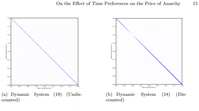
- In a two-action shared-resource model, exponential discounting can create multiple equilibria, some unstable, while the undiscounted game has only locally asymptotically stable equilibria; learning dynamics will accordingly behave differently.
Reading between the lines
- If the same model were run with agents whose discount functions are estimated experimentally, the predicted efficiency distribution would be bimodal: power-law discounters should cluster near PoA 2 while exponential discounters should show unbounded worst-case loss, independent of estimated discount parameters. This is a testable prediction the paper does not itself make.
- Because the social optimum is defined with an undiscounted long-run average, the paper measures efficiency from a patient planner's perspective; replacing that criterion with a discounted planner would likely compress the exponential-case loss and could break the power-law guarantee.
- For $\alpha\le 1$ the formal game's utility sum diverges, so the PoA=2 result tacitly adopts an overtaking or asymptotic-growth comparison; making that criterion explicit—or choosing a different tie-break—could change which stationary distributions count as equilibria.
- The stability contrast suggests that in real repeated-choice systems, exponential discounters may converge to low-efficiency equilibria, while power-law discounters should converge to the unique stable outcome; interventions that change the shape of agents' time preferences might therefore be more effective than adjusting incentives by a constant factor.
Signed reviews
Editorial analysis
A structured set of objections, weighed in public.
Referee Report
Summary. This paper studies a stateless mean-field congestion game in which a continuum of agents repeatedly choose actions with congestion-dependent sojourn times and maximize the discounted present value of an infinite reward stream. The paper defines stationary equilibria, proves existence for exponential discounting and for power-law discounting with α in [0,1], and computes the price of anarchy: infinity for exponential discounting and 2 for power-law discounting whenever a stationary equilibrium exists. It also analyzes stability under projection dynamics, showing that exponential discounting can create unstable equilibria while average-reward equilibria are always locally asymptotically stable.
Significance. If the results hold, the paper makes a clean and surprising contribution: the efficiency cost of selfish dynamic routing depends only on the qualitative form of time preference, not on its intensity. The exponential-discounting analysis is coherent and self-contained: existence via Kakutani's fixed point theorem, an equivalence to stable population games, and a sharp PoA expression in terms of a characteristic index. The stability comparison between discounted and undiscounted dynamics is also valuable, and the fixed-point and inequality arguments are reproducible from the text. However, the power-law α≤1 branch is currently not a theorem of the stated model, so the headline ''PoA = 2 whenever stationary equilibria exist'' is only conditionally established.
major comments (2)
- [§2, Eq. (1), Definition 1, §4.1, Theorem 2] The characterization of stationary equilibria for α≤1 is not derived from the model as stated. For α≤1 and any strategy that accrues infinitely many rewards, the sum in (1) diverges, so the supremum in (2) is attained by every such strategy and condition (6) in Definition 1 imposes no restriction on the stationary strategy σ†. The paper notices in §4.1 that 'the series diverges' and switches to the truncated comparison in (14), but no overtaking or catching-up optimality criterion is added to Definition 1. Consequently, Theorem 2's condition (15) does not follow from optimality, and the upper bound in Proposition 5, which uses (15), is not a consequence of the stated game. Concretely, take α=1/2, m=1, τ=(1,ε), r=(1,1/ε). Under the literal definition every stationary distribution is an equilibrium; the distribution μ=(1,0) is compatible and optimal, with SW=1, while the social optimum at μ=(0,1) has SW=1/ε², so the ratio is 1/ε²→∞, contradicting the PoA=2 claim. The model must either state an overtaking criterion explicitly or restrict the power-law results to α>1.
- [§4.3, Proposition 5, Appendix J] The upper-bound proof of Proposition 5 for α>1 relies on the assertion that at a stationary equilibrium 'it is optimal for the agents to choose the action with the largest possible reward rate' by Proposition 8. Proposition 8 establishes that a particular deterministic strategy is the unique best response after some initial time T, but it does not by itself show that this strategy maximizes the full infinite-horizon utility in (1); the proof in Appendix I compares rewards only from time T onward. Since Proposition 5 is the central efficiency claim for α>1, the argument needs to spell out why, if a stationary equilibrium exists, its optimal stationary strategy must coincide with the action identified by Proposition 8 on the entire horizon and why no nonstationary deviation during the initial period can improve on it.
minor comments (4)
- [§2 and §4] The power-law discounting parameter is introduced as α>0 in Section 2 but then stated as α≥0 in the first paragraph of Section 4; these should be made consistent.
- [§4.1, Eq. (14)] The displayed formula in (14) is typeset incorrectly: the summation limits involving T/τ_i appear garbled and the floor function is not rendered; please fix the notation.
- [Throughout] There are several typos that should be corrected: 'equilibirum' in Section 1, 'discouting' in Section 3.3, 'indepenedent' in the caption of Fig. 2, and 'The parameter are given as follows' in Section 5.3.
- [Appendix C] The proof of Theorem 1 asserts continuity of V∗(μ) in μ without proof; this is plausible under the standing assumptions but should be justified or cited.
Circularity Check
No circularity: the PoA theorems are derived from the stated equilibrium conditions and explicit constructions, with no fitted parameter renamed as prediction.
full rationale
The paper's central claims are derived rather than assumed. For exponential discounting, Theorem 1 characterizes equilibria via the fixed-point/Bellman condition (10), and Proposition 2 proves the PoA bound M+1 with an explicit lower-bound construction; Corollary 1 then follows by letting t2 grow. For power-law discounting, the PoA=2 upper bound in Proposition 5 is a direct inequality from Assumption 1 and the equilibrium support condition (15) (for alpha <= 1) or from Proposition 8's asymptotic best-response argument (for alpha > 1), and the lower bound is a constructed sequence with t1 -> 0. No fitted parameters are involved, and the PoA ratio is not used to define any equilibrium or payoff quantity. The no-discounting baseline from the authors' prior work [6] is re-derived in this paper for alpha = 0 via Theorem 2/Corollary 2, so the self-citation is not load-bearing. Section 4.1 does contain a genuine modeling gap: for alpha <= 1 the sum in (1) diverges, and the paper switches to the truncated-sum comparison (14), so the characterization (15) is not a consequence of Definition 1 as literally stated. This is a correctness/rigor risk, not a circularity: it does not make the PoA result an identity or convert an input into a prediction.
Assumptions & free parameters
assumptions (3)
- domain assumption Assumption 1: sojourn times are continuous and rate-monotone, i.e., if the rate of an action increases, its sojourn time cannot decrease.
- domain assumption The population of agents is a nonatomic continuum of constant mass, and strategies can be mixed.
- ad hoc to paper For power-law discounting with α≤1, 'optimal' means asymptotically optimal as the time horizon T→∞, rather than maximizing the divergent infinite sum in (1).
Cite this review
Pith. "Pith review of On the Effect of Time Preferences on the Price of Anarchy." pith.science (2026). https://pith.science/paper/5HOXG6EE
@misc{pith2026250420774,
  author       = {Pith},
  title        = {Pith review of: On the Effect of Time Preferences on the Price of Anarchy},
  year         = {2026},
  howpublished = {\url{https://pith.science/paper/5HOXG6EE}},
  note         = {Machine review of arXiv:2504.20774}
}
read the original abstract
This paper examines the impact of agents' myopic optimization on the efficiency of systems comprised by many selfish agents. In contrast to standard congestion games where agents interact in a one-shot fashion, in our model each agent chooses an infinite sequence of actions and maximizes the total reward stream discounted over time under different ways of computing present values. Our model assumes that actions consume common resources that get congested, and the action choice by an agent affects the completion times of actions chosen by other agents, which in turn affects the time rewards are accrued and their discounted value. This is a mean-field game, where an agent's reward depends on the decisions of the other agents through the resulting action completion times. For this type of game we define stationary equilibria, and analyze their existence and price of anarchy (PoA). Overall, we find that the PoA depends entirely on the type of discounting rather than its specific parameters. For exponential discounting, myopic behaviour leads to extreme inefficiency: the PoA is infinity for any value of the discount parameter. For power law discounting, such inefficiency is greatly reduced and the PoA is 2 whenever stationary equilibria exist. This matches the PoA when there is no discounting and players maximize long-run average rewards. Additionally, we observe that exponential discounting may introduce unstable equilibria in learning algorithms, if action completion times are interdependent. In contrast, under no discounting all equilibria are stable.
Figures


Figures from the paper (1 more)

Reference graph
Works this paper leans on
-
[1]
Journal of Economic Theory156, 269–316 (2015)
Adlakha, S., Johari, R., Weintraub, G.Y.: Equilibria of dynamic games with many players: Existence, approximation, and market structure. Journal of Economic Theory156, 269–316 (2015)
work page 2015
-
[2]
In: 2013 American Control Conference
Balandat, M., Tomlin, C.J.: On efficiency in mean field differential games. In: 2013 American Control Conference. pp. 2527–2532 (2013)
work page 2013
-
[3]
Banez, R.A., Li, L., Yang, C., Han, Z.: A Survey of Mean Field Game Applications in Wireless Networks, pp. 61–82. Springer International Publishing, Cham (2021)
work page 2021
-
[4]
Carmona, R., Graves, C.V., Tan, Z.: Price of anarchy for mean field games (2018)
work page 2018
-
[5]
Correa,J.,Cristi,A.,Oosterwijk,T.:Onthepriceofanarchyforflowsovertime.In:Proceedings of the 2019 ACM Conference on Economics and Computation. p. 559–577. EC ’19, Association for Computing Machinery, New York, NY, USA (2019)
work page 2019
-
[6]
Courcoubetis, C., Dimakis, A.: Stationary equilibrium of mean field games with congestion- dependent sojourn times. In: AAMAS ’23: Proceedings of the 20th International Conference on Autonomous Agents and MultiAgent Systems (2023)
work page 2023
-
[7]
Fischer, S., Vöcking, B.: On the evolution of selfish routing. In: Albers, S., Radzik, T. (eds.) Algorithms – ESA 2004. pp. 323–334. Springer Berlin Heidelberg, Berlin, Heidelberg (2004)
work page 2004
-
[8]
Gummadi, R., Johari, R., Schmit, S., Yu, J.Y.: Mean field analysis of multi-armed bandit games. SSRN (2013)
work page 2013
Show all 50 references
-
[9]
Math- ematics of Operations Research48(2), 656–686 (2023)
Guo, X., Hu, A., Xu, R., Zhang, J.: A general framework for learning mean-field games. Math- ematics of Operations Research48(2), 656–686 (2023)
2023
-
[10]
NeuroImage150, 336–343 (2017)
Hampton, W.H., Alm, K.H., Venkatraman, V., Nugiel, T., Olson, I.R.: Dissociable frontostriatal white matter connectivity underlies reward and motor impulsivity. NeuroImage150, 336–343 (2017)
2017
-
[11]
Journal of Economic Theory 144(4), 1665–1693.e4 (2009)
Hofbauer, J., Sandholm, W.H.: Stable games and their dynamics. Journal of Economic Theory 144(4), 1665–1693.e4 (2009)
2009
-
[12]
Econometrica60(5), 1127–1150 (1992)
Hopenhayn, H.A.: Entry, exit, and firm dynamics in long run equilibrium. Econometrica60(5), 1127–1150 (1992)
1992
-
[13]
Communications in Information & Systems6(3), 221–252 (2006)
Huang, M., Malhamé, R.P., Caines, P.E.: Large population stochastic dynamic games: closed- loop mckean-vlasov systems and the nash certainty equivalence principle. Communications in Information & Systems6(3), 221–252 (2006)
2006
-
[14]
Journal of Mathematical Eco- nomics 17(1), 77 – 87 (1988)
Jovanovic, B., Rosenthal, R.W.: Anonymous sequential games. Journal of Mathematical Eco- nomics 17(1), 77 – 87 (1988)
1988
-
[15]
Queueing Sys- tems 4(1), 69–76 (1989).https://doi.org/10.1007/BF01150857, https://doi.org/10.1007/ BF01150857
Kelly, F.P.: On a class of approximations for closed queueing networks. Queueing Sys- tems 4(1), 69–76 (1989).https://doi.org/10.1007/BF01150857, https://doi.org/10.1007/ BF01150857
1989 doi
-
[16]
Theory of Computing Systems 49(1), 71–97 (2011)
Koch, R., Skutella, M.: Nash equilibria and the price of anarchy for flows over time. Theory of Computing Systems 49(1), 71–97 (2011)
2011
-
[17]
Japanese Journal of Mathematics2(1), 229–260 (2007)
Lasry, J.M., Lions, P.L.: Mean field games. Japanese Journal of Mathematics2(1), 229–260 (2007)
2007
-
[18]
Springer New York, NY (1996)
Nagurney, A., Zhang, D.: Projected Dynamical Systems and Variational Inequalities with Ap- plications. Springer New York, NY (1996)
1996
-
[19]
Dynamic Games and Applications10(4), 845 – 871 (2020)
Neumann, B.A.: Stationary equilibria of mean field games with finite state and action space. Dynamic Games and Applications10(4), 845 – 871 (2020)
2020
-
[20]
Palgrave Macmillan (2013)
Pigou, A.C.: The economics of welfare. Palgrave Macmillan (2013)
2013
-
[21]
hyper- bolic
Prelec, D.: Decreasing impatience: A criterion for non-stationary time preference and “hyper- bolic” discounting. The Scandinavian Journal of Economics106(3), 511–532 (2004)
2004
-
[22]
18 (Routing Games)
Roughgarden, T.: Algorithmic Game Theory, chap. 18 (Routing Games). Cambridge University Press, 1st edn. (2007)
2007
-
[23]
ACM49(2), 236–259 (Mar 2002)
Roughgarden, T., Tardos, E.: How bad is selfish routing? J. ACM49(2), 236–259 (Mar 2002)
2002
-
[24]
The MIT Press (2010)
Sandholm, W.H.: Population Games and Evolutionary Dynamics. The MIT Press (2010)
2010
-
[25]
In: Zhou, Z
Wang, X., Jia, R.: Mean field equilibrium in multi-armed bandit game with continuous reward. In: Zhou, Z. (ed.) Proceedings of the Thirtieth International Joint Conference on Artificial Intelligence, IJCAI 2021, Virtual Event / Montreal, Canada, 19-27 August 2021. pp. 3118–
2021
-
[26]
∞X k=1 rake−β Pk j=1τaj (µ) # = nX i=1 σ1(i) rie−βτi(µ) + Eσ
Yardim, Batuhan, S.C., He, N.: Stateless mean-field games: A framework for independent learn- ingwithlargepopulations.In:SixteenthEuropeanWorkshoponReinforcementLearning(2023) A Motivating Example We consider a system where a common pool of agents choose between two inde- pend...
2023
-
[28]
Then, r1 τ1(µ† 1) − r2 τ2(µ† 1) = r1 t1 − r2 t2 = ≤ 0 if µ† 1 = 0 = 0 if µ† 1∈ (0,m ) ≥ 0 if µ† 1 =m If µ1 > 0 and µ1→ (µ† 1)+ where µ† 1∈ [0,m ), the constraint (17) is not tight at µ1 by continuity. It follows that (a) holds since r1 τ1(µ1)− r2 τ2(µ1) = r1 t1 − r2 t2...
-
[29]
Then, r1 τ1(µ† 1) − r2 τ2(µ† 1) = r1 t1 − r2 t2 = ≤ 0 if µ† 1 = 0 = 0 if µ† 1∈ (0,m ) ≥ 0 if µ† 1 =m Now we further assumeγ1 t1 − γ2 t2 > 0. 42 Y. Li et al. If µ1 > 0 and µ1→ (µ† 1)+ where µ† 1∈ [0,m ), the constraint (17) is still tight at µ1 since γ1 t1 − γ2 t2 > 0. ...
-
[30]
Then, r1 τ1(µ† 1) − r2 τ2(µ† 1) = r1 t1 +γ1w(µ† 1) − r2 t2 +γ2w(µ† 1) = ≤ 0 if µ† 1 = 0 = 0 if µ† 1∈ (0,m ) ≥ 0 if µ† 1 =m By continuity, the constraint (17) is always tight in a small neighborhood of the equilibrium pointµ†
-
[31]
Forµ1> 0 and µ1→ (µ† 1)+ or µ1→ (µ† 1)−, we have ¯g(µ1) := r1 τ1(µ1)− r2 τ2(µ1) = r1 t1 +γ1w(µ1)− r2 t2 +γ2w(µ1), where w(µ1)≥ 0 is the solution to the following equation regardingw, γ1 µ1 t1 +γ1w +γ2 m−µ1 t2 +γ2w =b. By Implicit Function Theorem and some algebra, the derivati...
-
[32]
< 0, forµ1→ (µ† 1)+, ¯g(µ†
-
[33]
Hence, (a) is true
< 0 by continuity. Hence, (a) is true. Assumeµ† 1 = m and ¯g(µ†
-
[34]
> 0, forµ1→ (µ† 1)−, ¯g(µ†
-
[35]
Hence, (b) is true
> 0 by continuity. Hence, (b) is true. Thus, we can assume¯g(µ†
-
[36]
= 0 at the equilibrium pointµ†
-
[37]
Then it suffices to show that ¯g(µ1) is decreasing inµ1 in a small neighborhood ofµ†
-
[38]
This is because if µ1→ (µ† 1)+, ¯g(µ1)≤ ¯g(µ†
-
[39]
= 0, (a) is true and ifµ1→ (µ† 1)−, ¯g(µ1)≥ ¯g(µ†
-
[40]
¯g(µ1) is indeed decreasing inµ1 in a small neighborhood ofµ†
= 0, (b) is true. ¯g(µ1) is indeed decreasing inµ1 in a small neighborhood ofµ†
-
[41]
=r1τ2(µ† 1), it follows that, ∂¯g ∂µ1 (µ†
-
[42]
=− r1τ2(µ† 1) γ2τ1(µ† 1)−γ1τ2(µ† 1) 2 γ2 2(m−µ† 1)(τ1(µ† 1))3τ2(µ†
-
[43]
We have shown that (a) and (b) are always true
+γ2 1µ† 1τ1(µ† 1)(τ2(µ† 1))3 , which is negative. We have shown that (a) and (b) are always true. Therefore, the set of equilibria of game¯F is locally asymptotically stable. L Proof of Proposition 7 We will only prove for one case of (20), i.e., γ1 γ2 > t1 t2 , γ1 γ2 < eβt1− ...
-
[44]
(48) Now we can choose(r1,r 2)∈ R2 + such that r1 eβτ1(µ† 1)− 1 = r2 eβτ2(µ† 1)− 1
respectively where w(µ† 1)≥ 0 is the is the solution to the following equation regardingw, γ1 µ† 1 t1 +γ1w +γ2 m−µ† 1 t2 +γ2w =b. (48) Now we can choose(r1,r 2)∈ R2 + such that r1 eβτ1(µ† 1)− 1 = r2 eβτ2(µ† 1)− 1 . (49) Hence, for anym > 0 and µ† 1∈ (0,m ), there exist (t1,t 2...
-
[45]
To proveµ† 1 is unstable, we only need to showgβ(µ1) is strictly increasing inµ1 in a small neighborhood ofµ†
= 0 andµ† 1 is an equilibrium. To proveµ† 1 is unstable, we only need to showgβ(µ1) is strictly increasing inµ1 in a small neighborhood ofµ†
-
[46]
Ifµ1 > µ† 1 and µ1 is close enough toµ† 1, gβ(µ1) > gβ(µ†
Assume this is true. Ifµ1 > µ† 1 and µ1 is close enough toµ† 1, gβ(µ1) > gβ(µ†
-
[47]
Ifµ1 <µ† 1 and µ1 is close enough to µ† 1, gβ(µ1) < gβ(µ†
= 0 , the mass flow will move towards action 1 under dynamic (18) andµ1 will continue to increase, which indicates thatµ† 1 is not stable. Ifµ1 <µ† 1 and µ1 is close enough to µ† 1, gβ(µ1) < gβ(µ†
-
[48]
It suffices to prove that∂gβ ∂µ1 (µ† 1)> 0
= 0, the mass flow will move towards action 2 under dynamic (18) andµ1 will continue to decrease, which also indicates thatµ† 1 is not stable. It suffices to prove that∂gβ ∂µ1 (µ† 1)> 0. By applying Implicit Function Theorem to w(µ1), which is the unique positive solution to e...
-
[49]
= τ1(µ† 1)τ2(µ† 1) γ1τ2(µ† 1)−γ2τ1(µ† 1) γ2 2(m−µ† 1)(τ1(µ† 1))2 +γ2 2µ† 1(τ2(µ† 1))2 · γ2r2βeβτ2(µ† 1) (eβτ2(µ† 1)− 1)2 − γ1r1βeβτ1(µ† 1) (eβτ1(µ† 1)− 1)2 ! = βτ1(µ† 1)τ2(µ† 1) γ1τ2(µ† 1)−γ2τ1(µ† 1) γ2 2(m−µ† 1)(τ1(µ† 1))2 +γ2 2µ† 1(τ2(µ† 1))2 · r1 eβτ1(µ† 1)− 1 · γ2eβτ2(µ† 1...
-
[50]
Therefore, µ† 1 is an unstable equilibrium ofFβ
=γ1(t2 +γ2w(µ† 1))−γ2(t1 +γ2w(µ† 1)) =γ1t2−γ2t1> 0, and γ2eβτ2(µ† 1) (eβτ2(µ† 1)− 1) − γ1eβτ1(µ† 1) (eβτ1(µ† 1)− 1) >γ 2−γ1 eβt1 eβt1− 1 > 0. Therefore, µ† 1 is an unstable equilibrium ofFβ
-
[3124]
Li et al
ijcai.org (2021) 20 Y. Li et al
2021
Reviewed August 16, 2026 · model on record in the stance chip above.
Discussion (0). Continue with ORCID to comment.