REVIEW 3 major objections 4 minor 2 cited by
Very massive stars at low metallicity: evolution, synthetic spectroscopy, and impact on the integrated light of starbursts
T0 review · 3 major / 4 minor · reviewed 2026-08-16 · deepseek-v4-flash
Pith's one-line read The paper argues that very massive stars at low metallicity retain a distinctive He II 1640 emission line in the integrated light of starbursts down to 0.1 solar metallicity, and that adding them hardens the ionizing spectrum below about…
desk verdict The paper convincingly shows HeII 1640 from VMS is a plausible low-metallicity tracer, but the 'survives down to 0.1 Zsun whatever the SFH' claim is bracketed by two mass-loss recipes that may not cover the real metallicity behavior. read the letter →
The pith
A machine-rendered reading of the paper's core claim, the machinery that carries it, and where it could break.
The reading
What carries the argument
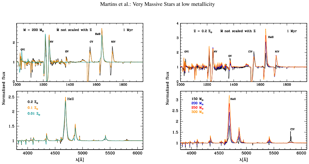
The machinery is a two-branch wind mass-loss recipe anchored on the empirical VMS calibration of Gräfener (2021): an optically thin branch and an optically thick branch, with the thick branch scaled by $(Z/Z_{\rm LMC})^x$ for $x=0$ or $x=1$. Stellar evolution tracks for initial masses 150, 200, 250 and 300 $M_\odot$ at $Z=0.2,0.1,0.01\,Z_\odot$ are computed with these recipes, and CMFGEN non-local thermodynamic equilibrium atmosphere models are made at selected ages using the predicted surface abundances, so the synthetic spectra and the population synthesis built from them are internally consistent. The argument-carrying observable is the He II 1640 emission line, formed in the dense winds of hot, helium-enriched VMS; its strength and profile track the stellar temperature, wind density, and surface composition across the model grid.
What would settle it
Observe a very young (≲1 Myr) massive cluster at Z ≈ 0.01 solar metallicity, for example a lensed low-metallicity star-forming galaxy that can be resolved into a compact cluster, and measure whether He II 1640 appears in emission in its integrated UV spectrum. A strong detection would rule out a linear or steeper metallicity scaling of VMS winds, because in those models the stars are too cool and their winds too weak to produce the line; a clean upper limit would rule out metallicity-independent winds, because those models keep the line strong at all ages.
Extended reading notes
Core claim
On the paper's own terms, the discovery is that the fate of a 150 to 300 solar mass star at low metallicity is decided by the wind mass-loss recipe. If VMS winds do not weaken with metallicity, the stars keep losing mass, stay near the zero-age main sequence for about 2.5 million years, and then evolve blueward; they remain hot, and their synthetic spectra show strong He II 1640 emission throughout. If the mass-loss rates scale linearly with metallicity, the weaker winds allow a helium II opacity bump to appear below the surface, the star inflates, and the track moves toward the red part of the Hertzsprung-Russell diagram; He II 1640 weakens and can disappear at 0.01 solar metallicity. In population synthesis, He II 1640 emission is present in integrated light at 0.2 and 0.1 solar metallicity for both burst and constant star formation histories, and also appears at 0.01 solar metallicity when winds are metallicity-independent. Adding VMS raises the number of ionizing photons below about 45 eV and boosts the ionizing photon efficiency, while the flux above 45 eV depends on age, metallicity, star formation history, and the shortest final phases of VMS evolution. The models reproduce the ultraviolet spectra of the low-metallicity starbursts II Zw 40-A, MrK71-A and SB 126 qualitatively and sometimes quantitatively, but the authors conclude that no clear choice between the two mass-loss frameworks emerges.
Load-bearing premise
The load-bearing premise is that the two adopted wind prescriptions bracket the true mass-loss behaviour of very massive stars below Large Magellanic Cloud metallicity, with the optically thin/thick wind transition left unchanged from the LMC calibration; no empirical constraint exists in that regime, and if the real metallicity dependence differs from zero or linear scaling, the evolutionary paths, the redward evolution, and the visibility of He II 1640 at 0.01 solar metallicity would change.
Editorial extensions
If this is right
- He II 1640 emission in an unresolved young starburst becomes a usable VMS tracer at metallicities down to at least 0.1 solar, for both burst and constant star formation histories; no resolved spectroscopy of individual stars is needed.
- At 0.01 solar metallicity, only the metallicity-independent wind family keeps the line strong, so a detection there would indicate that VMS winds scale with metallicity more weakly than linearly.
- Including VMS raises the number of ionizing photons below about 45 eV and raises the ionizing photon efficiency $\xi_{\rm ion}$, so high efficiencies measured in starburst galaxies no longer require a top-heavy initial mass function.
- The optical Wolf-Rayet bumps discriminate populations: the blue bump shows He II 4686 without N III 4634-42, and the red bump is a narrow C IV 5802-12 doublet, when VMS dominate instead of classical Wolf-Rayet stars.
- The short final hot phases of VMS barely affect the ultraviolet and optical integrated spectra, but they can raise $Q({\rm He\,II})/Q({\rm H\,I})$ to a few times $10^{-3}$, enough for nebular He II 4686 at roughly one percent of H$\beta$, yet not enough to explain the strongest observed He II emitters.
Reading between the lines
- If the true metallicity scaling is shallower than linear but not zero, VMS at 0.01 solar metallicity should show weak but detectable He II 1640 only at the youngest ages; stacking ultraviolet spectra of many low-metallicity star-forming regions could reveal this population-average line even where individual clusters are too faint.
- The two wind scenarios predict different surface nitrogen enhancement and different amounts of nitrogen ejected into the surroundings, so the nitrogen abundances of young low-metallicity systems, including the high-redshift N-emitters, may discriminate between them even when ultraviolet line ratios cannot.
- The models imply that the profile of He II 1640 becomes more purely emissive, with less P-Cygni absorption, as metallicity drops; equivalent-width thresholds for VMS selection should therefore be metallicity-dependent rather than fixed.
- The predictions above 45 eV rest on only a few sampled points in the final phases of VMS evolution, so the claimed nebular He II 4686 contribution is the least secure element of the hard-UV part of the model grid; a finer time sampling of the last 0.2 Myr would settle it.
Signed reviews
Editorial analysis
A structured set of objections, weighed in public.
Referee Report
Summary. Martins et al. compute evolutionary tracks for very massive stars (VMS) of 150-300 Msun at Z=0.2, 0.1 and 0.01 Zsun with the STAREVOL code, using two ad hoc metallicity scalings for optically thick VMS winds (no Z dependence, x=0, and linear Z dependence, x=1, in Eq. 2). They then compute CMFGEN non-LTE atmosphere models at selected ages along the tracks and include the resulting spectra in BPASS-based population synthesis models. The paper finds that VMS with Z-independent mass loss remain hot and near the ZAMS throughout their evolution, whereas VMS with linearly scaled mass loss evolve redward. VMS show HeII 1640 emission in most individual phases except when they become too cool, and this feature appears in integrated light down to 0.1 Zsun under most of the investigated configurations, though it is weaker or absent in the scaled mass-loss case at late ages. The models are compared to HST UV spectra of II Zw 40-A, MrK71-A and SB126, yielding qualitative and sometimes quantitative matches without clearly favouring either mass-loss prescription.
Significance. The paper provides a consistent and useful extension of VMS evolution, atmosphere and population-synthesis modelling to sub-LMC metallicities. Its central predictions, especially the behaviour of HeII 1640 and the increase in ionizing photons below about 45 eV when VMS are included, are falsifiable and can be confronted with existing and future UV spectroscopy of low-metallicity starbursts. A clear strength is the comparison with independent HST observations of three star-forming regions rather than a fit to the data used to calibrate the models. The authors are also transparent about the exploratory nature of the mass-loss assumptions and about the fact that their data cannot identify the preferred framework. The synthetic spectra are made publicly available on the POLLUX database, which aids reproducibility.
major comments (3)
- [Abstract; Sect. 2.1, Eq. (2); Sect. 5.3] The Abstract's claim that HeII 1640 is present in integrated light down to 0.1 Zsun 'whatever the star formation history' is not established for both adopted mass-loss prescriptions simultaneously. In the models with Z-scaled VMS mass loss, Sect. 4.2 states that HeII 1640 disappears at 2.5 Myr, and Sect. 4.3 reports that scaled-mass-loss burst models have almost no EW(HeII 1640) below Z=0.2 Zsun. The conclusion should be rephrased to make explicit which mass-loss framework, age range and detection criterion support the 'presence' claim, or the analysis should be repeated with a quantitative line-detection threshold rather than visual inspection.
- [Sect. 2.1, Eq. (2); Sect. 5.3] The two adopted wind prescriptions do not bracket the scenario in which the optically thin/thick wind transition itself shifts to higher luminosity at lower metallicity, as predicted by Sabhahit et al. (2023) and acknowledged by the authors in Sect. 5.3. If the transition moves in that direction, optically thick winds can be suppressed over much of the main sequence even for a linear Mdot(Z) scaling, leading to an earlier redward evolution than in the x=1 tracks. Because the HeII 1640 visibility of the integrated x=1 models already relies on the hottest early phases (the EW drops to near zero at ages near 2.5 Myr in Fig. 7, and to small values in CSF models after roughly 3 Myr), this unbracketed scenario could remove the feature at 0.1 Zsun. Including a third set of models with a metallicity-dependent thin/thick transition, or explicitly limiting the headline claim to the x=0 and x=1 frameworks, is necessary for the stated generality.
- [Sect. 4.3; Fig. 8] The paper uses the wording 'a weak emission is detected' for models where EW(HeII 1640) is close to zero after absorption lines over the 1625-1655 A window compensate the emission. This makes the central 'presence' claim difficult to evaluate quantitatively. I recommend defining a detection threshold based on line flux or on an EW significance criterion, so that statements such as 'present' or 'vanishes' are unambiguous across the different models and ages.
minor comments (4)
- [Fig. 20 caption] The caption gives 'Z=0.001 Zsun' for the orange lines, while the main text and Fig. 20 description refer to Z=0.01 Zsun; this appears to be a typo.
- [Table A.6] In the Z=0.01 Zsun scaled-mass-loss table, the 150 Msun model row at 2.50 Myr appears to have a malformed hydrogen abundance entry; the H and He columns should be checked.
- [Sect. 4.1] For ages 0 and 0.5 Myr the BPASS 1 Myr model is used for the normal-star population; this approximation is acknowledged in Sect. 4.6.2 for MrK71-A, but its systematic effect on the youngest burst comparisons in Figs. 15 and 16 is not quantified.
- [Abstract] The phrase 'whatever the star formation history' is stronger than what is computed; the authors consider one burst and one constant star-formation history built from discrete age bins, so a formulation such as 'for both the burst and constant star-formation histories considered here' would be more precise.
Circularity Check
No significant circularity: the HeII 1640 prediction is a forward-model output from evolutionary, atmosphere, and population-synthesis calculations, tested against external UV spectra rather than refit from them.
full rationale
The derivation chain is self-contained in the relevant sense. Stellar evolution models are computed with STAREVOL under two explicitly stated mass-loss frameworks (Sect. 2.1, Eqs. 1-2), with the Gräfener (2021) LMC calibration as the anchor and x=0 or x=1 for the metallicity scaling. These inputs determine the surface parameters along the tracks. CMFGEN atmosphere models then compute synthetic spectra from those parameters; HeII 1640 emission is an emergent radiative-transfer result, not a quantity fed into the evolution or into the mass-loss recipe. Population synthesis spectra are built by combining the VMS spectra with BPASS models (Sect. 4.1), and EW(HeII 1640) is measured from the resulting integrated spectra (Sect. 4.3). The paper does not fit HeII 1640 to the observed starbursts; it compares fixed model grids to II Zw 40-A, MrK71-A, and SB 126 (Sect. 4.6) and reports qualitative or partial quantitative agreement. The sample is admittedly selected on the presence of HeII 1640 in emission, which limits the strength of the observational test, but that selection does not make the model prediction circular. The paper explicitly states its central limitation: 'In absence of empirical constraint, we adopt two frameworks for the mass loss rates of VMS' and 'we are not able to clearly identify which mass loss framework is favoured.' This is an acknowledged uncertainty in the mass-loss prescription, not a circular reduction of the prediction to its inputs. Self-citations to Martins & Palacios (2022) supply the methodology and earlier LMC results, but the low-metallicity tracks, spectra, and population-synthesis predictions are newly computed here and are not justified by citing the earlier paper as the evidence for the low-Z conclusion. The robustness concern raised by the skeptic—that a metallicity-dependent thin/thick wind transition outside the x=0/x=1 envelope could alter the HeII 1640 visibility at 0.1 Zsun—is a real modeling uncertainty, acknowledged in Sect. 5.3, but it is a risk to the generality of the claim, not a circularity in the derivation.
Assumptions & free parameters
free parameters (4)
- VMS mass loss metallicity scaling exponent x =
0 or 1 (two scenarios)
- Wind clumping factor D =
10
- Ratio v_inf/v_esc =
2.6
- Upper IMF slope for normal stars =
-2.35
assumptions (4)
- domain assumption The Gräfener (2021) VMS mass loss recipe, calibrated in the LMC, applies unchanged at lower metallicity in the no-scaling scenario.
- ad hoc to paper The optically thin/thick wind transition condition of Gräfener (2021) does not vary with metallicity.
- domain assumption Solar-scaled chemical compositions and OPAL opacity tables are adequate at Z=0.01 Zsun, with no alpha-element enhancement except for a modest test.
- domain assumption BPASS models without binaries correctly represent the population of stars below 100 Msun.
Cite this review
Pith. "Pith review of Very massive stars at low metallicity: evolution, synthetic spectroscopy, and impact on the integrated light of starbursts." pith.science (2026). https://pith.science/paper/HNQECALI
@misc{pith2026250502993,
  author       = {Pith},
  title        = {Pith review of: Very massive stars at low metallicity: evolution, synthetic spectroscopy, and impact on the integrated light of starbursts},
  year         = {2026},
  howpublished = {\url{https://pith.science/paper/HNQECALI}},
  note         = {Machine review of arXiv:2505.02993}
}
read the original abstract
We study the spectroscopic appearance of very massive stars and their effect on the integrated light of starbursts at low metallicity (Z). We adopt two frameworks for the mass loss rates of VMS: in one case we assume no Z dependence, in the other case we assume a linear scaling with Z. We compute evolutionary models for masses 150, 200, 250 and 300 Msun at Z=0.2, 0.1 and 0.01 Zsun. We compute the associated synthetic spectra at selected points along the evolutionary tracks. Finally we build population synthesis models including VMS. We find that the evolution of VMS critically depends on the assumptions regarding mass loss rates. In case of no Z dependence VMS remain hot for all their lifetime. Conversely when mass loss rates are reduced because of lower Z VMS follow a classical evolution towards the red part of the HR diagram. VMS display HeII 1640 emission in most phases of their evolution, except when they become too cool. This line is present in the integrated light of population synthesis models down to 0.1 Zsun whatever the star formation history, and is also sometimes seen at Z=0.01 Zsun. HeII 1640 is weaker in models that include a Z scaling of the mass loss rates. The optical spectra of starbursts, especially the Wolf-Rayet bumps, sometimes display VMS signatures when these stars are present. At low Z, adding VMS to population synthesis models produces more ionising photons down to 45 eV. At higher energy the ionising flux depends on age, Z, assumption regarding VMS mass loss rates, and on the very short phases at the end of VMS evolution. HeII ionising fluxes large enough to produce some amount of nebular HeII 4686 emission can be produced under specific circumstances. Our models are able to reproduce qualitatively and sometimes also quantitatively the UV spectra of star-forming regions. However we are not able to clearly identify which mass loss framework is favoured.
Figures


Figures from the paper (17 more)


Forward citations
Cited by 2 Pith papers
-
SPURS: Massive Stars, Dense Gas, and Ly$\alpha$ Escape in GN-z11 at $z = 10.6$
GN-z11's rest-UV spectrum shows young massive stars with very massive star winds, dense gas, and a broad red Ly alpha wing that may help Ly alpha escape the largely neutral early universe.
-
pySTARBURST99: The Next Generation of STARBURST99
A Python rewrite of STARBURST99 with new low-metallicity and very massive star models predicts a 0.3 dex boost in HI ionising flux when the upper mass limit is raised from 120 to 300 solar masses.
Reference graph
Works this paper leans on
-
[1]
, " * write output.state after.block = add.period write newline
ENTRY address archiveprefix author booktitle chapter edition editor howpublished institution eprint journal key month note number organization pages publisher school series title type volume year label extra.label sort.label short.list INTEGERS output.state before.all mid.sentence after.sentence after.block FUNCTION init.state.consts #0 'before.all := #1 ...
-
[2]
write newline
" write newline "" before.all 'output.state := FUNCTION n.dashify 't := "" t empty not t #1 #1 substring "-" = t #1 #2 substring "--" = not "--" * t #2 global.max substring 't := t #1 #1 substring "-" = "-" * t #2 global.max substring 't := while if t #1 #1 substring * t #2 global.max substring 't := if while FUNCTION word.in bbl.in " " * FUNCTION format....
-
[3]
J., & Scott , P
Asplund , M., Grevesse , N., Sauval , A. J., & Scott , P. 2009, , 47, 481
2009
-
[4]
M., & Hamann , W
Barniske , A., Oskinova , L. M., & Hamann , W. R. 2008, , 486, 971
2008
-
[5]
Bestenlehner , J. M. 2020, , 493, 3938
2020
-
[6]
M., Crowther , P
Bestenlehner , J. M., Crowther , P. A., Caballero-Nieves , S. M., et al. 2020, , 499, 1918
2020
-
[7]
M., Gr \"a fener , G., Vink , J
Bestenlehner , J. M., Gr \"a fener , G., Vink , J. S., et al. 2014, , 570, A38
2014
-
[8]
M., Vink , J
Bestenlehner , J. M., Vink , J. S., Gr \"a fener , G., et al. 2011, , 530, L14
2011
Show all 102 references
-
[9]
A., de Koter , A., Bestenlehner , J
Brands , S. A., de Koter , A., Bestenlehner , J. M., et al. 2022, , 663, A36
2022
-
[10]
& Charlot , S
Bruzual , G. & Charlot , S. 2003, , 344, 1000
2003
-
[11]
J., Saxena , A., Cameron , A
Bunker , A. J., Saxena , A., Cameron , A. J., et al. 2023, , 677, A88
2023
-
[12]
J., Katz , H., Rey , M
Cameron , A. J., Katz , H., Rey , M. P., & Saxena , A. 2023, , 523, 3516
2023
-
[13]
2009, , 499, 279
Cantiello , M., Langer , N., Brott , I., et al. 2009, , 499, 279
2009
-
[14]
P., Mathis , J
Cassinelli , J. P., Mathis , J. S., & Savage , B. D. 1981, Science, 212, 1497
1981
-
[15]
2024, , 972, 143
Castellano , M., Napolitano , L., Fontana , A., et al. 2024, , 972, 143
2024
-
[16]
I., Abbott , D
Castor , J. I., Abbott , D. C., & Klein , R. I. 1975, , 195, 157
1975
-
[17]
2023, , 673, L7
Charbonnel , C., Schaerer , D., Prantzos , N., et al. 2023, , 673, L7
2023
-
[18]
2024, , 976, L15
Chemerynska , I., Atek , H., Dayal , P., et al. 2024, , 976, L15
2024
-
[19]
2023, Nature Astronomy, 7, 771
Chen , Y., Jones , T., Sanders , R., et al. 2023, Nature Astronomy, 7, 771
2023
-
[20]
Conti , P. S. & Morris , P. W. 1990, , 99, 898
1990
-
[21]
A., Caballero-Nieves , S
Crowther , P. A., Caballero-Nieves , S. M., Bostroem , K. A., et al. 2016, , 458, 624
2016
-
[22]
Crowther , P. A. & Castro , N. 2024, , 527, 9023
2024
-
[23]
A., Dessart , L., Hillier , D
Crowther , P. A., Dessart , L., Hillier , D. J., Abbott , J. B., & Fullerton , A. W. 2002, , 392, 653
2002
-
[24]
A., Schnurr , O., Hirschi , R., et al
Crowther , P. A., Schnurr , O., Hirschi , R., et al. 2010, , 408, 731
2010
-
[25]
J., Stanway , E
Eldridge , J. J., Stanway , E. R., Xiao , L., et al. 2017, , 34, e058
2017
-
[26]
J., Groh , J
Farrell , E. J., Groh , J. H., Meynet , G., et al. 2020, , 495, 4659
2020
-
[27]
V., Schlosser , W., Schmidt-Kaler , T., & Winkler , C
Feitzinger , J. V., Schlosser , W., Schmidt-Kaler , T., & Winkler , C. 1980, , 84, 50
1980
-
[28]
Figer , D. F. 2005, , 434, 192
2005
-
[29]
P., Chisholm , J., et al
Fujimoto , S., Naidu , R. P., Chisholm , J., et al. 2025, arXiv e-prints (ApJ submitted), arXiv:2501.11678
2025 arXiv
-
[30]
2021, , 647, A13
Gr \"a fener , G. 2021, , 647, A13
2021
-
[31]
& Hamann , W
Gr \"a fener , G. & Hamann , W. R. 2008, , 482, 945
2008
-
[32]
2021, , 647, A99
Grassitelli , L., Langer , N., Mackey , J., et al. 2021, , 647, A99
2021
-
[33]
G., Izotov , Y
Guseva , N. G., Izotov , Y. I., & Thuan , T. X. 2000, , 531, 776
2000
-
[34]
2015, , 581, A21
Hainich , R., Pasemann , D., Todt , H., et al. 2015, , 581, A21
2015
-
[35]
2014, , 565, A27
Hainich , R., R \"u hling , U., Todt , H., et al. 2014, , 565, A27
2014
-
[36]
R., Gr \"a fener , G., & Liermann , A
Hamann , W. R., Gr \"a fener , G., & Liermann , A. 2006, , 457, 1015
2006
-
[37]
R., Gr \"a fener , G., Liermann , A., et al
Hamann , W. R., Gr \"a fener , G., Liermann , A., et al. 2019, , 625, A57
2019
-
[38]
R., Vink , J
Higgins , E. R., Vink , J. S., Hirschi , R., Laird , A. M., & Sabhahit , G. N. 2023, , 526, 534
2023
-
[39]
Hillier , D. J. & Miller , D. L. 1998, , 496, 407
1998
-
[40]
Hummer , D. G. & Storey , P. J. 1987, , 224, 801
1987
-
[41]
2023, , 959, 100
Isobe , Y., Ouchi , M., Tominaga , N., et al. 2023, , 959, 100
2023
-
[42]
I., Foltz , C
Izotov , Y. I., Foltz , C. B., Green , R. F., Guseva , N. G., & Thuan , T. X. 1997, , 487, L37
1997
-
[43]
L., Tsamis , Y
James , B. L., Tsamis , Y. G., Barlow , M. J., et al. 2009, , 398, 2
2009
-
[44]
2024, , 535, 881
Ji , X., \"U bler , H., Maiolino , R., et al. 2024, , 535, 881
2024
-
[45]
M., Horch , E
Kalari , V. M., Horch , E. P., Salinas , R., et al. 2022, , 935, 162
2022
-
[46]
M., Guerrero , M
Kehrig , C., V \' lchez , J. M., Guerrero , M. A., et al. 2018, , 480, 1081
2018
-
[47]
M., P \'e rez-Montero , E., et al
Kehrig , C., V \' lchez , J. M., P \'e rez-Montero , E., et al. 2015, , 801, L28
2015
-
[48]
2015, , 573, A71
K \"o hler , K., Langer , N., de Koter , A., et al. 2015, , 573, A71
2015
-
[49]
P., Pauldrach , A., Puls , J., & Abbott , D
Kudritzki , R. P., Pauldrach , A., Puls , J., & Abbott , D. C. 1989, , 219, 205
1989
-
[50]
1992, , 265, L17
Langer , N. 1992, , 265, L17
1992
-
[51]
C., & Levesque , E
Leitherer , C., Byler , N., Lee , J. C., & Levesque , E. M. 2018, , 865, 55
2018
-
[52]
C., & Faisst , A
Leitherer , C., Lee , J. C., & Faisst , A. 2019, , 158, 192
2019
-
[53]
1987, , 178, 159
Maeder , A. 1987, , 178, 159
1987
-
[54]
2020, , 499, L105
Marques-Chaves , R., \'A lvarez-M \'a rquez , J., Colina , L., et al. 2020, , 499, L105
2020
-
[55]
2021, , 507, 524
Marques-Chaves , R., Schaerer , D., \'A lvarez-M \'a rquez , J., et al. 2021, , 507, 524
2021
-
[56]
2022, , 517, 2972
Marques-Chaves , R., Schaerer , D., \'A lvarez-M \'a rquez , J., et al. 2022, , 517, 2972
2022
-
[57]
2024, , 681, A30
Marques-Chaves , R., Schaerer , D., Kuruvanthodi , A., et al. 2024, , 681, A30
2024
-
[58]
2023, , 679, A137
Martinet , S., Meynet , G., Ekstr \"o m , S., Georgy , C., & Hirschi , R. 2023, , 679, A137
2023
-
[59]
J., Paumard , T., et al
Martins , F., Hillier , D. J., Paumard , T., et al. 2008, , 478, 219
2008
-
[60]
& Palacios , A
Martins , F. & Palacios , A. 2022, , 659, A163
2022
-
[61]
2023, , 678, A159
Martins , F., Schaerer , D., Marques-Chaves , R., & Upadhyaya , A. 2023, , 678, A159
2023
-
[62]
L., Lee , J
Maschmann , D., Leitherer , C., Faisst , A. L., Lee , J. C., & Minsley , R. 2024, , 961, 159
2024
-
[63]
2023, , 269, 33
Nakajima , K., Ouchi , M., Isobe , Y., et al. 2023, , 269, 33
2023
-
[64]
Osterbrock , D. E. & Ferland , G. J. 2006, Astrophysics of gaseous nebulae and active galactic nuclei
2006
-
[65]
F., & Tsang , B
Pascale , M., Dai , L., McKee , C. F., & Tsang , B. T. H. 2023, , 957, 77
2023
-
[66]
2016, , 456, 4191
Patr \' cio , V., Richard , J., Verhamme , A., et al. 2016, , 456, 4191
2016
-
[67]
2000, , 141, 23
Puls , J., Springmann , U., & Lennon , M. 2000, , 141, 23
2000
-
[68]
E., Furlanetto , S
Robertson , B. E., Furlanetto , S. R., Schneider , E., et al. 2013, , 768, 71
2013
-
[69]
N., Vink , J
Sabhahit , G. N., Vink , J. S., Higgins , E. R., & Sander , A. A. C. 2022, , 514, 3736
2022
-
[70]
N., Vink , J
Sabhahit , G. N., Vink , J. S., Sander , A. A. C., et al. 2025, , 696, A200
2025
-
[71]
N., Vink , J
Sabhahit , G. N., Vink , J. S., Sander , A. A. C., & Higgins , E. R. 2023, , 524, 1529
2023
-
[72]
R., & Todt , H
Sander , A., Hamann , W. R., & Todt , H. 2012, , 540, A144
2012
-
[73]
Sander , A., Todt , H., Hainich , R., & Hamann , W. R. 2014, , 563, A89
2014
-
[74]
Sander , A. A. C. 2024, in IAU Symposium, Vol. 361, Massive Stars Near and Far, ed. J. Mackey , J. S. Vink , & N. St-Louis , 473--478
2024
-
[75]
Sander , A. A. C. & Vink , J. S. 2020, , 499, 873
2020
-
[76]
2002, , 382, 28
Schaerer , D. 2002, , 382, 28
2002
-
[77]
Schaerer , D., Fragos , T., & Izotov , Y. I. 2019, , 622, L10
2019
-
[78]
2025, , 693, A271
Schaerer , D., Guibert , J., Marques-Chaves , R., & Martins , F. 2025, , 693, A271
2025
-
[79]
2024, , 687, L11
Schaerer , D., Marques-Chaves , R., Xiao , M., & Korber , D. 2024, , 687, L11
2024
-
[80]
N., Moffat , A
Schnurr , O., Casoli , J., Chen \'e , A. N., Moffat , A. F. J., & St-Louis , N. 2008, , 389, L38
2008
-
[81]
Seaton , M. J. 1978, , 185, 5P
1978
-
[82]
Seeyave , L. T. C., Wilkins , S. M., Kuusisto , J. K., et al. 2023, , 525, 2422
2023
-
[83]
P., et al
Senchyna , P., Plat , A., Stark , D. P., et al. 2024, , 966, 92
2024
-
[84]
P., Charlot , S., et al
Senchyna , P., Stark , D. P., Charlot , S., et al. 2021, , 503, 6112
2021
-
[85]
A., et al
Shenar , T., Sana , H., Crowther , P. A., et al. 2023, , 679, A36
2023
-
[86]
J., Crowther , P
Smith , L. J., Crowther , P. A., Calzetti , D., & Sidoli , F. 2016, , 823, 38
2016
-
[87]
J., Oey , M
Smith , L. J., Oey , M. S., Hernandez , S., et al. 2023, , 958, 194
2023
-
[88]
2015, , 576, A83
Stasi \'n ska , G., Izotov , Y., Morisset , C., & Guseva , N. 2015, , 576, A83
2015
-
[89]
2006, , 132, 253
Stolte , A., Brandner , W., Brandl , B., & Zinnecker , H. 2006, , 132, 253
2006
-
[90]
2024, , 686, A185
Upadhyaya , A., Marques-Chaves , R., Schaerer , D., et al. 2024, , 686, A185
2024
-
[91]
2023, , 678, A173
Vanzella , E., Loiacono , F., Bergamini , P., et al. 2023, , 678, A173
2023
-
[92]
Villar-Mart \' n , M., Cervi \ n o , M., & Gonz \'a lez Delgado , R. M. 2004, , 355, 1132
2004
-
[93]
Vink , J. S., ed. 2015, Astrophysics and Space Science Library, Vol. 412, Very Massive Stars in the Local Universe , ed. J. S. Vink
2015
-
[94]
Vink , J. S. 2023, , 679, L9
2023
-
[95]
S., de Koter , A., & Lamers , H
Vink , J. S., de Koter , A., & Lamers , H. J. G. L. M. 2001, , 369, 574
2001
-
[96]
Vink , J. S. & Gr \"a fener , G. 2012, , 751, L34
2012
-
[97]
S., Muijres , L
Vink , J. S., Muijres , L. E., Anthonisse , B., et al. 2011, , 531, A132
2011
-
[98]
2014, , 781, 122
Wofford , A., Leitherer , C., Chandar , R., & Bouret , J.-C. 2014, , 781, 122
2014
-
[99]
2023, , 523, 3949
Wofford , A., Sixtos , A., Charlot , S., et al. 2023, , 523, 3949
2023
-
[100]
2021, , 500, 2908
Wofford , A., Vidal-Garc \' a , A., Feltre , A., et al. 2021, , 500, 2908
2021
-
[101]
L., & Arnould , M
Xu , Y., Goriely , S., Jorissen , A., Chen , G. L., & Arnould , M. 2013, , 549, A106
2013
-
[102]
2013, , 433, 1114
Yusof , N., Hirschi , R., Meynet , G., et al. 2013, , 433, 1114
2013
Reviewed August 16, 2026 · model on record in the stance chip above.
Discussion (0). Continue with ORCID to comment.