REVIEW 4 major objections 5 minor 22 references
Physics-Informed DeepONets for drift-diffusion on metric graphs: simulation and parameter identification
T0 review · 4 major / 5 minor · reviewed 2026-08-15 · deepseek-v4-flash
Pith's one-line read Three operator-learning surrogate networks, one per edge type, trained once and coupled through vertex flux conditions, solve the nonlinear drift-diffusion equation on metric graphs and recover unknown initial conditions and velocities…
desk verdict A genuinely novel forward-surrogate method with an under-specified inverse section and a load-bearing low-dimensional coupling ansatz. read the letter →
The pith
A machine-rendered reading of the paper's core claim, the machinery that carries it, and where it could break.
The reading
What carries the argument
The load-bearing object is the triple of physics-informed DeepONet operators $\mathcal{G}^{\text{inflow}}$, $\mathcal{G}^{\text{inner}}$, and $\mathcal{G}^{\text{outflow}}$. Each DeepONet maps a vector of sensor measurements, $u^{\text{sensor}}=(u^{\text{origin}},u^{\text{target}},u^{\text{init}},\nu_e)$, to the space-time density $\mathcal{G}^{u_{\text{sensor}}}_\theta(t,x)$ on one edge of its type, with a physics residual enforcing the drift-diffusion equation and edge-specific boundary losses enforcing the inflow, inner, or outflow flux condition. The machinery that assembles edges into a graph is the coupling loss $$L_{\text{coupling}}(z)=\frac{1}{|V_K|}\sum_{v\in V_K}\frac{1}{|E_v|}\sum_{e,e'\in E_v}(\hat\$rho_e^{{u(z)}}$(t_i,v)-\hat\rho_{e'}^{u(z)}(t_i,v))^2+\frac{1}{|V_K|}\sum_{v\in V_K}\frac{1}{|E_v|}\Big(\sum_{e\in E_v}\hat $J_e^{{u(z)}}$(t_i,v)n_e(v)\Big)^2,$$ whose first sum enforces continuity of densities at every interior vertex and whose second sum enforces mass conservation through the Kirchhoff-Neumann condition. To keep the minimization cheap, the unknown vertex fluxes are parameterized as $z(t)=\sum_{k=1}^{10}\beta_k\exp(-|t-t_k|^2/\ell^2)$ with $\ell=0.2$, reducing the graph coupling to a few dozen coefficients $\beta_k$ optimized by gradient descent; augmenting the same loss with measured density and flux residuals converts it into the inverse-problem objective. A DeepONet is an operator network that learns a map from input functions to solution functions rather than a single function.
What would settle it
Run the coupled framework on a graph whose vertex flux is a fast oscillating function, say $z(t)=\sin(40\pi t)$ on $[0,1]$, well outside the span of ten RBF centers with $\ell=0.2$, and compare the coupling loss and final $L^2$ error with the smooth-Gaussian-process cases; if the errors stay near $10^{-3}$ to $10^{-2}$, the RBF restriction is not limiting, while if they jump by orders of magnitude the claim is restricted to smooth fluxes.
Extended reading notes
Core claim
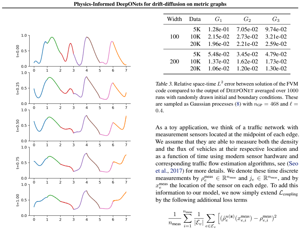
The central claim is that the map from boundary data to the solution of the nonlinear drift-diffusion equation $H(\rho_e)=\partial_t\rho_e-\partial_x(\varepsilon\partial_x\rho_e-\nu_e f(\rho_e))=0$, with $f(\rho)=\rho(1-\rho)$ and vertex conditions (5) and (4), factorizes through three edge operators. DeepONet models $\mathcal{G}^{\text{inflow}}$, $\mathcal{G}^{\text{inner}}$, and $\mathcal{G}^{\text{outflow}}$ are trained once, graph-agnostically, on representative inflow, inner, and outflow edges; any metric graph is then assembled by treating each edge as one of these three types and minimizing a coupling loss over the unknown vertex flux functions $z(t)$. The coupling loss enforces continuity of $\rho$ at each interior vertex and the Kirchhoff-Neumann flux condition $\sum_{e\in E_v} J_e(v)n_e(v)=0$, with $z(t)$ restricted to the class $z(t)=\sum_{k=1}^{10}\beta_k\exp(-|t-t_k|^2/\ell^2)$, $\ell=0.2$. On three small test graphs the coupled forward solutions have absolute $L^2$ errors of $4.68\times 10^{-3}$ to $5.81\times 10^{-3}$ (relative $1.06\times 10^{-2}$ to $1.30\times 10^{-2}$); on a 1034-edge graph the forward relative error is $4.84\times 10^{-2}$. For the inverse problem, adding density- and flux-misfit terms to the same coupling loss recovers unknown initial conditions and edge velocities, with relative errors of $3.53\times 10^{-2}$ for the reconstructed solution and $2.34\times 10^{-2}$ for the velocities on the large graph. The paper's claim is that forward simulation and parameter identification on coupled networks therefore become the same computational task.
Load-bearing premise
The load-bearing premise is that every unknown time-dependent flux at a graph vertex, and therefore the initial conditions and velocities recovered in the inverse problem, can be represented well by a smooth bell-shaped interpolation using only ten fixed-width centers, so if a true physical flux has sharper or more complex time structure than this ten-term family allows, the coupled solution and the recovered parameters will be biased regardless of how accurate the edge surrogate networks are.
Editorial extensions
If this is right
- A newly specified graph requires no retraining of the edge models: only the vertex-coupling coefficients are optimized, so simulation cost grows roughly linearly with the number of edges rather than quadratically, as the paper estimates for a classical finite-volume inverse solve.
- Parameter identification costs about the same as a forward run, because unknown initial conditions, edge velocities, and vertex fluxes all enter the same low-dimensional coefficient vector and are recovered by adding data-misfit terms to the coupling loss.
- The trained surrogates generalize across graph sizes: the same three models that give errors near $10^{-2}$ on small test graphs achieve a relative forward error of $4.84\times 10^{-2}$ on a graph with 1034 edges.
- The recovered initial conditions and per-edge velocities from noisy synthetic sensor data retain the essential space-time structure of the solution, which the paper identifies as a step toward real-time traffic-state estimation.
Reading between the lines
- The paper fixes every training edge to length one, so a natural but untested extension is rescaling or retraining edge surrogates for non-unit edge lengths before the claim of arbitrary metric graphs is fully exercised; the current evidence covers unit-length edges with varying topology.
- The ten-center RBF ansatz for vertex fluxes is the most likely point where real data would strain the method: measured traffic fluxes have sharp rush-hour transients that a fixed-width ten-term smooth interpolation cannot represent, so testing on the open traffic datasets the paper cites would show whether the inverse-problem accuracy is an artifact of smooth synthetic data.
- The same Lego-style coupling should transfer to other graph PDEs—the paper itself points to gas-network and intracellular-transport equations—and the transferable part is the vertex-coupling loss, which only needs the edge surrogates' flux evaluations; a concrete test would be swapping the drift-diffusion residual for a hyperbolic traffic model and checking whether the vertex coupling still conver
Signed reviews
Editorial analysis
A structured set of objections, weighed in public.
Referee Report
Summary. The paper proposes a physics-informed DeepONet framework for the nonlinear drift-diffusion equation on metric graphs. Three edge surrogate models are trained once for inflow, inner, and outflow edges using a physics-informed residual loss and boundary/initial data from a finite volume solver. At evaluation time, the surrogates are coupled by enforcing continuity and Kirchhoff conditions at vertices, where the unknown vertex fluxes are represented by a fixed 10-term RBF ansatz. The same coupling loss is extended with sensor data misfit terms to solve inverse problems for unknown initial conditions and edge velocities. The paper reports absolute L2 errors in the range 4.68e-3 to 5.81e-3 on three small test graphs, a relative error of 4.84e-2 on a 1034-edge graph, and inverse-problem errors in Tables 4 and 5. The manuscript also contains a well-developed existence/uniqueness proof for the continuous problem and a mass-conserving, bound-preserving finite volume discretization.
Significance. If the central claims are substantiated, the method would be a genuinely useful operator-learning framework for graph-coupled PDEs: after a one-time training of three edge surrogates, arbitrary graph topologies can be assembled by solving a small coupling optimization, and inverse problems are handled by adding loss terms rather than by repeated forward solves. The paper has clear strengths: the analysis in Section 2 and Appendix A provides a rigorous weak-solution theory; the finite volume scheme in Appendix B comes with mass-conservation and bound-preservation proofs; and the deliberate use of different Gaussian-process parameters for training, simulation, and inverse tests (Section 3 and Appendix C.1) shows awareness of inverse-crime issues. The significance is currently tempered by three gaps: the low-dimensional RBF ansatz for all vertex fluxes, the missing parameterization of the unknown fields in the inverse problem, and the absence of an independent verification reference. These gaps affect the reported error numbers and the generality of the claims, but they are addressable with additional experiments and exposition.
major comments (4)
- [Section 4, Eq. (10) and following paragraph] The entire coupling mechanism is restricted to vertex fluxes z(t) of the form sum_{k=1}^{10} beta_k exp(-|t-t_k|^2/0.04), with fixed centers and width l=0.2. The paper provides no evidence that vertex fluxes arising from the drift-diffusion equation on arbitrary graphs lie in this 10-dimensional space. Since L_coupling is minimized only over these beta coefficients, any component of the true vertex flux outside this ansatz cannot be resolved, and the coupling loss cannot vanish even if the edge surrogates are perfect. This is load-bearing because the ansatz supplies the only degrees of freedom through which the three edge models communicate. The absence of a direct comparison between the reconstructed z(t) and the FVM vertex flux is a concrete gap; such a comparison, together with a test whose true flux is not in the RBF class (for example, a time variation shorter than the length scale l=0.2, or a flux drawn from a different stochastic model), is needed to support the error claims in Tables 2, 3, and the large-graph results in Appendix E.
- [Section 5, paragraph beginning 'As a toy application'] The inverse-problem section states that after optimizing the augmented L_coupling, 'evaluating the vector u' recovers the unknown initial condition and the edge velocities nu_e, but it never states how these unknowns are parameterized. If they are encoded through the same 10-center, l=0.2 RBF ansatz introduced in Section 4, then all inverse results are conditional on that ansatz; if they are encoded differently, the text must say how. Moreover, no identifiability or regularization discussion is given for recovering an edge-dependent velocity and a generally non-smooth initial condition from pointwise sensor data. Without this parameterization, the headline statement that the inverse problem costs practically the same as the forward problem is not fully interpretable, and the 'err. init.' and 'err. vel.' columns in Tables 4 and 5 cannot be reproduced or judged.
- [Section 3, paragraph 'To generate training data...'] The training protocol fixes l_e=1 and T=1 but never specifies the values of the diffusion constant epsilon and the velocities nu_e used in the finite volume solves that generate the training data. Since Eq. (1) contains these parameters and the inverse problem seeks nu_e, the trained surrogates are meaningful only for the particular epsilon and nu_e range used in training; the test graphs and the large graph in Appendix E should state these values. In addition, the claim of applicability to 'arbitrary metric graphs' requires an explanation of how a surrogate trained on unit intervals is evaluated on edges of different length, since the metric graph setting explicitly allows edge-dependent lengths l_e.
- [Tables 2-5 and Appendix E] All reference solutions reported in the numerical sections are produced by the finite volume solver described in Appendix B, which is also the source of the boundary and vertex-flux data used in training the edge surrogates. This is self-referential benchmarking: agreement with the FVM reference does not exclude errors shared between the surrogate and the FVM discretization. A single comparison against an independent reference, such as a manufactured analytic solution or a distinctly discretized solver on one of the test graphs, would materially strengthen the evidence for the headline accuracy claims.
minor comments (5)
- [Section 3, after the outflow loss formula] The outflow edge loss is labeled Linflow_edge in the text; it should be Loutflow_edge to match the nomenclature used for the other two edge types.
- [Appendix B.1, Eqs. (24) and (25)] The symbol de(t) appears without definition in the finite volume derivation; the authors should clarify whether it is a directional indicator, a typographical artifact, or an otherwise intended factor in the convective flux.
- [Section 4, after Eq. (10)] The kernel width is stated as l=0.2 after the formula z(t)=sum_{k=1}^{n_beta} beta_k phi(t-t_k), but the relation between n_beta and the previously chosen value 10 should be made explicit in one place, rather than only in the surrounding prose.
- [Software and Data section] The sentence 'If the paper is accepted, we publish all software and data...' should be unconditional if the authors intend to release code, or should state explicitly what will be withheld and why, so that reviewers and readers can verify the results.
- [Figure 7 caption] The phrase 'in the eye ball norm' is informal; the authors should replace it with a precise quantitative error measure or define the visual comparison being made.
Circularity Check
No circular reduction found; the RBF coupling ansatz is a restrictive approximation, not a circular input, and the FVM self-citation is non-load-bearing.
full rationale
The claimed derivation chain is not circular. The edge DeepONets are trained with a PDE residual loss plus initial and flux boundary sensor terms, and the flux sensor values for inner edges are obtained from the authors' finite volume implementation. Although Appendix B says the FVM was 'previously introduced in (Blechschmidt et al., 2022)', that self-citation is not load-bearing: the present paper restates the full finite-volume discretization and proves mass conservation and bound preservation (Theorem B.1), with convergence support from independent classical references (LeVeque, 2002; Lazarov et al., 1996; Morton et al., 1997; ten Thije Boonkkamp & Anthonissen, 2010). The FVM is therefore an external, described reference solver rather than an unexamined self-citation. The coupling step in Section 4 introduces the RBF ansatz z(t) = sum_k beta_k exp(-|t-t_k|^2/l^2) with n_beta=10 and l=0.2. This is a finite-dimensional restriction on the unknown vertex fluxes, and it is indeed the main approximation weakness of the method, but it is not circular: the coupled solution is not defined to be the RBF fit itself; it is the minimizer of the continuity and Kirchhoff losses under that ansatz. The numerical validation uses test initial and boundary data drawn from a Gaussian process with nGP=468 and l=0.4, while the training data use nGP=512 and l=0.5, so the benchmark is not the same function instances used for fitting. In the inverse setting, the unknown initial conditions and velocities are recovered by minimizing data misfit plus coupling losses; Appendix C.1 explicitly discloses the strong prior (l=0.2, 10 centers) used for the inverse problem. That disclosure shows an identifiability/approximation limitation, not an equivalence of the recovered parameters to the data by construction. No prediction in the paper reduces to its own input by definition, and the only self-citation is minor and non-load-bearing; hence the score is 2 rather than 0.
Assumptions & free parameters
free parameters (10)
- Diffusion constant epsilon
- Edge length =
1 (fixed for all edges)
- Time horizon =
1 (fixed)
- RBF length scale for training-data GP =
0.5
- Number of GP centers for training data =
512
- RBF length scale for test/simulation GP =
0.4
- Number of GP centers for test data =
468
- RBF length scale for coupling flux representation =
0.2
- Number of RBF centers for coupling flux representation =
10
- FVM numerical flux stabilization parameter =
1 (in Theorem B.1)
assumptions (6)
- domain assumption Existence, uniqueness, and a priori bounds (0 <= rho <= 1) of the weak solution to the drift-diffusion graph problem.
- standard math The DeepONet architecture can approximate the PDE solution operator on each edge to the required accuracy.
- domain assumption The in-house finite volume solver is convergent and produces correct reference solutions.
- ad hoc to paper Vertex fluxes at coupling nodes can be represented by z(t) = sum_{k=1}^{10} beta_k exp(-|t-t_k|^2 / 0.04).
- domain assumption Training data are representative of the distribution of all admissible initial and boundary conditions on graphs.
- domain assumption The velocity nu_e is well-defined as an operator input and is covered by the training distribution.
Cite this review
Pith. "Pith review of Physics-Informed DeepONets for drift-diffusion on metric graphs: simulation and parameter identification." pith.science (2026). https://pith.science/paper/DYQGSXRN
@misc{pith2026250504263,
  author       = {Pith},
  title        = {Pith review of: Physics-Informed DeepONets for drift-diffusion on metric graphs: simulation and parameter identification},
  year         = {2026},
  howpublished = {\url{https://pith.science/paper/DYQGSXRN}},
  note         = {Machine review of arXiv:2505.04263}
}
read the original abstract
We develop a novel physics informed deep learning approach for solving nonlinear drift-diffusion equations on metric graphs. These models represent an important model class with a large number of applications in areas ranging from transport in biological cells to the motion of human crowds. While traditional numerical schemes require a large amount of tailoring, especially in the case of model design or parameter identification problems, physics informed deep operator networks (DeepONet) have emerged as a versatile tool for the solution of partial differential equations with the particular advantage that they easily incorporate parameter identification questions. We here present an approach where we first learn three DeepONet models for representative inflow, inner and outflow edges, resp., and then subsequently couple these models for the solution of the drift-diffusion metric graph problem by relying on an edge-based domain decomposition approach. We illustrate that our framework is applicable for the accurate evaluation of graph-coupled physics models and is well suited for solving optimization or inverse problems on these coupled networks.
Figures


Figures from the paper (9 more)




Reference graph
Works this paper leans on
-
[1]
Finally, using once more the definition ofwk, cf
A similar argument implies that the outflow terms are bounded as well. Finally, using once more the definition ofwk, cf. Eq (13), we further estimate the second term in (20), using the weighted Young inequality, X e∈E Z le 0 Z Ω ρk e (1−ρk e)|∂xwk|2 dx≥ X e∈E Z le 0 |∂xρk e|2 ρke(1−ρke) dx− 2 Z le 0 |νe||∂xρk e|dx + Z le 0 ρk e (1−ρk e)ν2 e dx ! ≥ X e∈E Z...
work page 2010
-
[3]
doi: 10.1088/0951-7715/29/11/3528. WWU::123155. Burger, M., Humpert, I., and Pietschmann, J.-F. On Fokker- Planck equations with in- and outflow of mass. Kinetic & Related Models, 13:249–277, 01
-
[7]
A deep learning framework for solution and discovery in solid mechanics
Haghighat, E., Raissi, M., Moure, A., Gomez, H., and Juanes, R. A deep learning framework for solution and discovery in solid mechanics. arXiv:2003.02751,
arXiv 2003
-
[8]
Solid lines report training loss of various terms, dashed lines report validation loss
Terms of loss function in training of models with width 100 and 5K (up), 10K (middle), 20K (down) training data. Solid lines report training loss of various terms, dashed lines report validation loss. Recall that although only PDE physics loss ( pde ph log), boundary physics loss (bnd ph log) and initial condition loss (ics log) are considered in objectiv...
work page 2021
-
[10]
1103/physrevlett.114.168101. URL http://dx.doi. org/10.1103/PhysRevLett.114.168101. Brezis, H. Functional Analysis, Sobolev Spaces and Partial Differential Equations. Springer Science and Business Media, Berlin Heidelberg,
-
[11]
doi: 10.1038/s41598-019-51539-5
ISSN 2045-2322. doi: 10.1038/s41598-019-51539-5. Lu, L., Jin, P., Pang, G., Zhang, Z., and Karniadakis, G. E. Learning nonlinear operators via deeponet based on the universal approximation theorem of operators. Nature machine intelligence, 3(3):218–229,
-
[12]
doi: https://doi.org/10.1016/j.cma.2019. 112789. Meng, X. and Karniadakis, G. E. A composite neural net- work that learns from multi-fidelity data: Application to function approximation and inverse PDE problems. Journal of Computational Physics, 401,
-
[13]
S., Venzke, A., and Chatzivasileiadis, S
Misyris, G. S., Venzke, A., and Chatzivasileiadis, S. Physics-informed neural networks for power systems. In 2020 IEEE Power & Energy Society General Meeting (PESGM), pp. 1–5. IEEE,
work page 2020
Show all 22 references
-
[14]
Raissi, M., Yazdani, A., and Karniadakis, G. E. Hidden fluid mechanics: A navier-stokes informed deep learn- ing framework for assimilating flow visualization data. arXiv:1808.04327,
-
[15]
Physics informed deep learning for computational elastodynamics without labeled data
Rao, C., Sun, H., and Liu, Y . Physics informed deep learning for computational elastodynamics without labeled data. arXiv:2006.08472,
2006 arXiv
-
[17]
Proof of Theorem 2.2 The proof is based on extending ideas from (Gomes et al., 2019; Burger et al., 2020), where in- and outflow boundary conditions are treated, to metric graphs
11 Physics-Informed DeepONets for drift-diffusion on metric graphs A. Proof of Theorem 2.2 The proof is based on extending ideas from (Gomes et al., 2019; Burger et al., 2020), where in- and outflow boundary conditions are treated, to metric graphs. We will work with Sobolev s...
2019
-
[19]
These are popular discretization schemes as they usually work in a structure preserving manner
is used which was previously introduced in (Blechschmidt et al., 2022). These are popular discretization schemes as they usually work in a structure preserving manner. B.1. Finite volume scheme To derive a finite volume scheme we briefly recall our setup and start from conside...
2022
-
[20]
To solve the system of ordinary differential equations (26) for the unknowns ρe k andρv, respectively, we introduce the following time-discretization
(26d) In (26b) accumulated contributions evaluated inv vanish due to the Kirchhoff-Neumann vertex conditions (4). To solve the system of ordinary differential equations (26) for the unknowns ρe k andρv, respectively, we introduce the following time-discretization. For some equ...
1997
-
[21]
With similar arguments like before we conclude that the right-hand side is non- negative and thus, 1−⃗ ρn≥ 0, which proves the upper bound
Due tof(x) =x(1−x) we may rewrite (28) in the form (M +τεA )(⃗1−⃗ ρn) =M(⃗1−⃗ ρn−1) +⃗G(⃗1−⃗ ρn−1), with some vector-valued function ⃗G. With similar arguments like before we conclude that the right-hand side is non- negative and thus, 1−⃗ ρn≥ 0, which proves the upper bound. ...
2023
-
[2002]
Neural operator: Graph kernel network for partial differential equations
Li, Z., Kovachki, N., Azizzadenesheli, K., Liu, B., Bhat- tacharya, K., Stuart, A., and Anandkumar, A. Neural operator: Graph kernel network for partial differential equations. arXiv preprint arXiv:2003.03485,
2003 arXiv
-
[2006]
Universal differential equations for scientific machine learning
Rackauckas, C., Ma, Y ., Martensen, J., Warner, C., Zubov, K., Supekar, R., Skinner, D., Ramadhan, A., and Edelman, A. Universal differential equations for scientific machine learning. arXiv preprint arXiv:2001.04385,
2001 arXiv
-
[2011]
and Karniadakis, G
Jagtap, A. and Karniadakis, G. Extended physics-informed neural networks (XPINNs): A generalized space-time do- main decomposition based deep learning framework for nonlinear partial differential equations. Communications in Computational Physics, 28:2002–2041, 11
2002
-
[2016]
URL https://dx.doi.org/10.1088/ 1751-8113/49/34/345602
doi: 10.1088/1751-8113/49/34/ 345602. URL https://dx.doi.org/10.1088/ 1751-8113/49/34/345602. Bressloff, P. C. and Levien, E. Synaptic democracy and vesicular transport in axons. Physical Review Letters, 114(16),
-
[2017]
doi: https://doi.org/10.1016/j.arcontrol.2017
ISSN 1367-5788. doi: https://doi.org/10.1016/j.arcontrol.2017. 03.005. Simon, J. Compact sets in the space Lp(O,T ;B). Annali di Matematica pura ed applicata, 146:65–96,
2017 doi
-
[2019]
Gyrya, V
doi: 10.1137/18M1215980. Gyrya, V . and Zlotnik, A. An explicit staggered-grid method for numerical simulation of large-scale natural gas pipeline networks. Applied Mathematical Modelling, 65:34–51,
-
[2020]
doi: 10.3934/krm. 2020009. Chen, X., Duan, J., and Karniadakis, G. E. Learning and meta-learning of stochastic advection-diffusion-reaction systems from sparse measurements. European Journal of Applied Mathematics , 32(3):397–420,
-
[2025]
doi: https://doi.org/10.1016/j.jde.2025.02
ISSN 0022-0396. doi: https://doi.org/10.1016/j.jde.2025.02
2025 doi
Reviewed August 15, 2026 · model on record in the stance chip above.
Discussion (0). Continue with ORCID to comment.