REVIEW 3 major objections 5 minor 49 references
Robust computation of higher-dimensional invariant tori from individual trajectories
T0 review · 3 major / 5 minor · reviewed 2026-08-15 · deepseek-v4-flash
Pith's one-line read A single short trajectory can determine a higher-dimensional invariant torus without initial guesses or continuation.
desk verdict A practically valuable pipeline for computing higher-dimensional invariant tori from single short trajectories, with an honest but real theoretical gap in the frequency-convergence step. read the letter →
The pith
A machine-rendered reading of the paper's core claim, the machinery that carries it, and where it could break.
The reading
What carries the argument
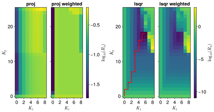
The load-bearing object is the Birkhoff reduced rank extrapolation (Birkhoff RRE) filter: a palindromic set of coefficients $c_j$ that extrapolates the trajectory, whose residual $R_{\mathrm{RRE}}$ classifies the trajectory as integrable or chaotic, and whose filter roots $\psi_j$ produce high-accuracy frequency estimates $\Omega_j\approx\omega\cdot k_j$. Around this sit two further mechanisms: a Bayesian maximum a posteriori estimator that assigns wavenumbers to the measured frequencies and recovers a valid rotation vector, and a Korkine-Zolatarev lattice reduction on the averaged metric $G=\sum_k \|h_k\|^2 kk^\top$ that selects the homology generators giving the most compact Fourier representation. The final least-squares coefficient fit is what converts the trajectory and rotation vector into an explicit torus parameterization.
What would settle it
Run the frequency-extraction step on a trajectory of a known smooth two-dimensional torus with a prescribed rotation vector, increasing the filter size $J$, and check whether the computed frequencies approach the exact values $\omega\cdot k$; the central claim fails if the top frequencies plateau away from machine precision or never contain a pair of wavenumbers with determinant $\pm1$.
Extended reading notes
Core claim
The central claim is that the rotation vector and Fourier parameterization of a $d$-dimensional invariant torus can be recovered from a single finite trajectory, without continuation or initial guesses, by combining temporal frequency estimation with a Bayesian labeling of wavenumbers. Specifically, Birkhoff RRE returns high-precision frequencies $\Omega_j$ and magnitudes $H_j$; the MAP step identifies which lattice wavenumbers $k_j$ produced those frequencies and thereby finds a valid rotation vector $\omega$; the KZ reduction replaces $\omega$ by an equivalent rotation vector whose loops on the torus are short and nearly orthogonal; and a least-squares fit of the trajectory against modes $e^{2\pi i k\cdot\theta}$ yields the torus Fourier coefficients. The authors demonstrate the pipeline on random initial conditions of a weakly coupled standard map, on island chains, and on three-dimensional tori in the Earth-Moon restricted three-body problem, reporting KAM residuals as low as $3.63\times10^{-6}$ with trajectory lengths on the order of $10^3$--$10^4$.
Load-bearing premise
The whole method rests on an unproved assumption: the frequencies that the extrapolation step returns really converge to the true frequencies of the torus for tori of dimension two or higher, and the strongest recovered frequencies contain enough independent directions to form a valid rotation vector.
Editorial extensions
If this is right
- For the weakly coupled standard map with 1000 random initial conditions, 851 trajectories are classified as integrable by length 8001, and 95 percent of the initialized tori are successfully parameterized by the reported a posteriori measure.
- The method computes three-dimensional tori of the Earth-Moon restricted three-body problem from trajectories of length 3335 to 8335, with KAM residuals of $3.63\times10^{-6}$, $5.70\times10^{-6}$, and $1.63\times10^{-5}$.
- Birkhoff reduced rank extrapolation classifies the standard-map trajectories as integrable with roughly an order of magnitude shorter trajectories than weighted Birkhoff averaging requires.
- The main failure modes are nearly resonant rotation vectors and strongly filamentary tori; the authors show these are detectable through the KAM residual and resonance-order diagnostics.
- Island-chain trajectories are handled by treating the chain period as an added rational frequency, so a single pipeline covers tori, islands, and chaotic classification.
Reading between the lines
- If a convergence proof for the frequency roots were supplied, the Bayesian uncertainty $\sigma_\omega$ could be set from theory, which would turn the pipeline into a method with end-to-end error estimates for the recovered torus.
- Because only injectivity of the observable $h(S)$ is required, the same steps should work with delay embeddings or other observables, extending the method to systems whose natural state space is not Euclidean.
- Since trajectory generation is often the dominant cost, the short-trajectory property suggests this approach could map out many tori in parameter scans where continuation-based methods struggle.
- The KZ step is a lattice shortest-vector problem on the torus's average metric; the same reduction could be used to identify slow and fast directions in higher-dimensional systems for model reduction.
Signed reviews
Editorial analysis
A structured set of objections, weighed in public.
Referee Report
Summary. The paper proposes a fully data-driven method for computing invariant tori of dimension d > 1 from a single, relatively short trajectory, without continuation or an initial guess. The pipeline has four stages: (i) Birkhoff reduced rank extrapolation (RRE) to extract many temporal frequencies and their amplitudes from the trajectory; (ii) a Bayesian maximum a posteriori (MAP) problem, Eq. (25), that selects a valid rotation vector from among the measured frequencies; (iii) a Korkine-Zolotarev lattice reduction that chooses a homology basis adapted to the shape of the torus; and (iv) an adaptive least-squares Fourier parameterization, Eq. (7) and Sec. 2.2. The method is tested on a coupled standard map (1000 random initial conditions, with 851 classified as integrable), on island chains, and on three three-dimensional tori in the cislunar elliptic restricted three-body problem. The authors report KAM residuals RKAM between 3.63e-6 and 1.63e-5 for the 3D examples and a 95% success rate for the standard-map ensemble, and they discuss two failure modes: nearly resonant rotation vectors and highly anisotropic (filamentary) tori.
Significance. If the central claims hold, this would be a practically valuable tool for astrodynamics and plasma physics, since it removes the need for continuation or a good initial guess and works from a single trajectory, including for tori of dimension three. The paper's strengths are its honest validation methodology: the KAM residual in Eq. (29) is evaluated on a uniform grid rather than on the fitting trajectory, and the validation error Rh in Eq. (9) uses held-out trajectory points. The authors also explicitly acknowledge the main theoretical gap, namely that convergence of Birkhoff RRE frequencies to the true Fourier frequencies omega·k is unproven for d > 1. The numerical experiments are extensive and the code is publicly available in SymplecticMapTools.jl. The main risk is that the entire method depends on that unproven convergence, and the reported residuals, while encouraging, are integrated checks that do not isolate whether the frequency estimates converge.
major comments (3)
- [Sec. 3.1 and Sec. 5] The load-bearing assumption of the method is that the Birkhoff RRE frequencies Omega_j converge to the true temporal frequencies omega·k_j for d > 1. The paper explicitly states in Sec. 3.1 that 'There is currently no theory for the convergence of the frequencies Omega_j to true values omega·k_j as J→∞' and repeats in the Conclusion that this is an open question. The MAP step in Sec. 3.2, Eq. (25), takes the measured Omega_j as input and restricts candidate rotation vectors to subsets of Omega, so if this convergence fails, the method collapses even on a perfectly smooth torus. The empirical evidence in Sec. 4 is integrated: the reported RKAM residuals are computed with the same estimated frequencies used to construct the parameterization, and a wrong but nearby frequency could still yield small residuals on a finite trajectory sampled on a 25×25 grid. I therefore ask for a targeted numerical test that isolates frequency convergence, for example comparing Birkhoff RRE frequencies against frequencies obtained from a high-accuracy parameterization-method torus for one or two d = 2 and d = 3 examples, with controlled J, T, and analytic or high-precision ground truth. Without such a test, the central methodological claim is not fully supported.
- [Sec. 3.2, Eq. (20) and Eq. (25)] The prior hyperparameters C and r in sigma(k) = C e^{-r||k||} are fit by least squares to the same trajectory's sorted Fourier magnitudes H_j, Eq. (20), and then used as the prior in the MAP objective (25). This is an empirical-Bayes procedure that uses the data twice: the same trajectory both determines the prior and is the evidence in the posterior. This double use can overstate posterior confidence and may bias the wavenumber assignment toward the fitted smoothness model. The paper does not report sensitivity of the final rotation vector or RKAM to changes in C and r, nor does it compare with a fixed, cross-validated choice. I request a sensitivity study that perturbs the fitted C and r (or holds out a fraction of the H_j when fitting them) and reports how often the rotation vector and the final RKAM change. The order-statistic model in Eq. (22) also assumes no measurement error in the H_j, which is an additional idealization that should be stated and tested.
- [Sec. 4.1, Fig. 7 caption and Introduction] The paper claims in the Introduction that 'we successfully parameterize 95% of the initialized tori for the weakly coupled standard map,' but the success criterion is not defined: no threshold on RKAM (or Rh) is given, and it is unclear whether the denominator is 1000 initialized trajectories, the 851 classified as integrable, or the 853 appearing in the Fig. 7 caption. The count inconsistency (851 in the text versus 853 in the caption) also needs correction. Since this 95% claim is a headline result, the definition of success and the exact counts must be made precise and reproducible.
minor comments (5)
- [Abstract and Sec. 3.3] The name 'Korkine-Zolatarev' is a misspelling; the standard spelling is Korkine-Zolotarev.
- [Sec. 2.1, Eq. (9)] The definition of R_h^2 writes R2_h = 1/R2_h0 sum ||h(F^t(x)) - hat h(theta + omega t)||^2, but the second factor R2_h0 is defined immediately after; please make the dependence on the theta initialization explicit, since the expression as written is ambiguous.
- [Sec. 3.4] In the sentence 'Typical values of these constants are pmax = 10 and epsilon_ada = 10^-8,' the symbol epsilon_ada appears to be a typo for epsilon_isl, which is the island tolerance defined earlier in the same paragraph.
- [Sec. 2.3] There is a duplicated word in 'a resolution of (K1, K2) = (24, 18) would be needed to capture all of the same Fourier modes for for the sheared torus.'
- [Sec. 4.1, Fig. 6] The statement that 'the weighted Birkhoff classification rate approximately matches the Birkhoff RRE classification rate in the right panel' is made without a quantitative comparison; reporting the actual classification counts for the weighted Birkhoff average at the same trajectory lengths would make the comparison in Fig. 6 more informative.
Circularity Check
No definitional circularity; one mild empirical-Bayes double-use in the MAP prior, while the rotation-vector search and KAM validation are independent.
-
other
[Section 3.2, Eqs. (20)-(25)]
"To find these parameters, consider the idealized case that H consist of a sorted list of the exact expected norms H2 k = E[∥hk∥2] = Dσ(k)2. ... we heuristically fit a line to the log-norm of the coefficients H ... (20) ... αj(Hj,π(j)) = P(H2 π(j)=H2 j)/P(H2 π(j)≤H2 J0). (25)"
The same sorted magnitudes H_j are used twice: first to calibrate the smoothness-prior hyperparameters C and r in Eq. (20), and then as the 'data' in the likelihood ratio α_j in Eq. (25). Thus the Bayesian prior is not independent of the observations it scores; it is an empirical-Bayes fit to the very H_j used in the MAP objective. This is a mild in-sample calibration rather than a definitional equivalence: the frequency likelihood P(Ω_j|ω,π(j)) with very small σω dominates the label assignment, and the det±1 and KZ checks enforce that the selected pair is a genuine integer homology change. The final KAM residual is also an independent uniform-grid check, so this double-use does not force the central claim.
full rationale
The central derivation is self-contained. Birkhoff RRE solves the constrained least-squares problem (17)-(18) for a filter, and the frequencies Ω_j are roots of the associated linear difference equation, not a fitted parameter renamed as output. The MAP step (25) combines these measured frequencies with a smoothness prior; the only in-sample element is Eq. (20), where C and r are fit to the same H_j that Eq. (25) later scores via α_j. This is an empirical-Bayes double-use, but it does not determine the rotation vector by itself. The frequency likelihood with σω of order 10^-10 dominates the label assignment, and the det±1 condition plus KZ reduction ensure that the selected pair is a genuine integer change of homology. The final parameterization is validated with the held-out trajectory error Rh (9) and the uniform-grid KAM residual RKAM (29), both independent of the least-squares fit. The paper's own admission that convergence of the Birkhoff RRE roots to ω·k for d>1 is open (Sec. 3.1 and Sec. 5) is a rigor gap, not circularity, because the method does not assume that theorem as an input. Accordingly, the only mild circularity signal is the fitted smoothness prior, worth a 2 rather than a higher score.
Assumptions & free parameters
free parameters (6)
- Prior decay rate r and scale C in sigma(k) = C e^{-r||k||} =
Fit by linear regression to the trajectory's sorted Fourier magnitudes (Eq. 20)
- MAP frequency uncertainty sigma_omega =
Chosen as 1e-10 in Sec. 4.1; range 1e-7 to 1e-11 suggested in Sec. 3.2
- Number of frequencies J0 used in MAP =
30 for standard map (Sec. 4.1); 20, 18, 8 for ER3BP examples
- Wavenumber search bound P =
Scales as gamma (J0)^(1/d) with gamma about 10
- Birkhoff RRE filter length J and trajectory length T =
Chosen per example; default (J, T) = (2000, 4000) for standard map; (2500, 3334) for L4 ER3BP
- Maximum Fourier modes Kmax =
2000 (Sec. 4.1)
assumptions (7)
- domain assumption Diophantine condition on the rotation vector omega
- domain assumption Smoothness, analytic or C^M, of the torus and observable with rapidly decaying Fourier coefficients
- domain assumption Injectivity of the observable embedding h(S)
- ad hoc to paper Uniform prior on the rotation vector and independence assumptions in the Bayesian model
- standard math Birkhoff ergodic theorem and convergence of weighted Birkhoff averages
- ad hoc to paper Existence of a valid rotation vector among the observed frequency set Omega
- ad hoc to paper Order-statistic model with no measurement error on the coefficient magnitudes
Cite this review
Pith. "Pith review of Robust computation of higher-dimensional invariant tori from individual trajectories." pith.science (2026). https://pith.science/paper/TEJGKMQU
@misc{pith2026250508715,
  author       = {Pith},
  title        = {Pith review of: Robust computation of higher-dimensional invariant tori from individual trajectories},
  year         = {2026},
  howpublished = {\url{https://pith.science/paper/TEJGKMQU}},
  note         = {Machine review of arXiv:2505.08715}
}
read the original abstract
We present a method for computing invariant tori of dimension greater than one. The method uses a single short trajectory of a dynamical system without any continuation or initial guesses. No preferred coordinate system is required, meaning the method is practical for physical systems where the user does not have much \textit{a priori} knowledge. Three main tools are used to obtain the rotation vector of the invariant torus: the reduced rank extrapolation method, Bayesian maximum a posteriori estimation, and a Korkine-Zolatarev lattice basis reduction. The parameterization of the torus is found via a least-squares approach. The robustness of the algorithm is demonstrated by accurately computing many two-dimensional invariant tori of a standard map example. Examples of islands and three-dimensional invariant tori are shown as well.
Figures


Figures from the paper (7 more)


Reference graph
Works this paper leans on
-
[1]
Carl D. Murray and Stanley F. Dermott. Solar System Dynamics . Cambridge University Press, Cam- bridge, 2000
work page 2000
-
[2]
R. D. Hazeltine and J. D. Meiss. Plasma confinement. Dover Publications, Mineola, N.Y, 2003
work page 2003
-
[3]
An Introduction to Stellarators: From Magnetic Fields to Symmetries and Optimization
Lise-Marie Imbert-Gerard, Elizabeth Paul, and Adelle Wright. An Introduction to Stellarators: From Magnetic Fields to Symmetries and Optimization . Society for Industrial and Applied Mathematics, Philadelphia, PA, 2024
work page 2024
-
[4]
Alex Haro, Marta Canadell, Jordi-Lluis Figueras, Alejandro Luque, and Josep Maria Mondelo. The Parameterization Method for Invariant Manifolds: From Rigorous Results to Effective Computations , volume 195 of Applied Mathematical Sciences. Springer International Publishing, Cham, 2016
work page 2016
-
[5]
A. Haro and R. de la Llave. A parameterization method for the computation of invariant tori and their whiskers in quasi-periodic maps: Rigorous results. Journal of Differential Equations , 228(2):530–579, September 2006. 31
work page 2006
-
[6]
Alex Haro and Rafael de la Llave. A parameterization method for the computation of invariant tori andtheir whiskers in quasi-periodic maps: Numerical algorithms. Discrete and Continuous Dynamical Systems - B , 6(6):1261–1300, August 2006
work page 2006
-
[7]
A. Haro and R. de la Llave. A Parameterization Method for the Computation of Invariant Tori and Their Whiskers in Quasi-Periodic Maps: Explorations and Mechanisms for the Breakdown of Hyperbolicity. SIAM Journal on Applied Dynamical Systems , 6(1):142–207, January 2007
work page 2007
-
[8]
Rafael de la LLave. A tutorial on KAM theory . American Mathematical Society; Oxford University Press, Providence, R.I., Oxford, 2004
work page 2004
Show all 49 references
-
[9]
On conservation of conditionally periodic motions for a small change in Hamilton’s function
Andrey Nikolaevich Kolmogorov. On conservation of conditionally periodic motions for a small change in Hamilton’s function. In Dokl. akad. nauk Sssr , volume 98, pages 527–530, 1954
1954
-
[10]
Proof of a theorem of AN Kolmogorov on the invariance of quasi-periodic motions under small perturbations of the Hamiltonian
Vladimir I Arnold. Proof of a theorem of AN Kolmogorov on the invariance of quasi-periodic motions under small perturbations of the Hamiltonian. Collected Works: Representations of Functions, Celestial Mechanics and KAM Theory, 1957–1965 , pages 267–294, 2009
1957
-
[11]
On invariant curves of area-preserving mappings of an annulus
Jurgen M¨ oser. On invariant curves of area-preserving mappings of an annulus. Nachr. Akad. Wiss. G¨ ottingen, II, pages 1–20, 1962
1962
-
[12]
Figueras, A
J.-Ll. Figueras, A. Haro, and A. Luque. Rigorous Computer-Assisted Application of KAM Theory: A Modern Approach. Foundations of Computational Mathematics , 17(5):1123–1193, October 2017
2017
-
[13]
Olikara, and Daniel J
Nicola Baresi, Zubin P. Olikara, and Daniel J. Scheeres. Fully Numerical Methods for Continuing Families of Quasi-Periodic Invariant Tori in Astrodynamics. The Journal of the Astronautical Sciences , 65(2):157–182, June 2018
2018
-
[14]
Jeremy Kasdin, and Pini Gurfil
Egemen Kolemen, N. Jeremy Kasdin, and Pini Gurfil. Multiple Poincar´ e sections method for finding the quasiperiodic orbits of the restricted three body problem. Celestial Mechanics and Dynamical Astronomy, 112(1):47–74, January 2012
2012
-
[15]
On the computation of reducible invariant tori on a parallel computer
Angel Jorba and Estrella Olmedo. On the computation of reducible invariant tori on a parallel computer. SIAM Journal on Applied Dynamical Systems , 8(4):1382–1404, 2009
2009
-
[16]
Leveraging quasi-periodic orbits for trajectory design in cislunar space
Brian P McCarthy and Kathleen C Howell. Leveraging quasi-periodic orbits for trajectory design in cislunar space. Astrodynamics, 5(2):139–165, 2021
2021
-
[17]
R. L. Dewar and J. D. Meiss. Flux-minimizing curves for reversible area-preserving maps. Physica D: Nonlinear Phenomena, 57(3):476–506, August 1992
1992
-
[18]
R. L. Dewar, S. R. Hudson, and P. F. Price. Almost invariant manifolds for divergence-free fields. Physics Letters A , 194(1):49–56, October 1994
1994
-
[19]
S. R. Hudson and R. L. Dewar. Almost-invariant surfaces for magnetic field-line flows. Journal of Plasma Physics, 56(2):361–382, October 1996
1996
-
[20]
S. R. Hudson, D. A. Monticello, and A. H. Reiman. Reduction of islands in full-pressure stellarator equilibria. Physics of Plasmas , 8(7):3377–3381, July 2001
2001
-
[21]
Direct com- putation of magnetic surfaces in Boozer coordinates and coil optimization for quasisymmetry
Andrew Giuliani, Florian Wechsung, Georg Stadler, Antoine Cerfon, and Matt Landreman. Direct com- putation of magnetic surfaces in Boozer coordinates and coil optimization for quasisymmetry. Journal of Plasma Physics , 88(4):905880401, August 2022
2022
-
[22]
Introduction to Frequency Map Analysis
Jacques Laskar. Introduction to Frequency Map Analysis. In Carles Sim´ o, editor,Hamiltonian Systems with Three or More Degrees of Freedom, pages 134–150. Springer Netherlands, Dordrecht, 1999
1999
-
[23]
J. Laskar. The chaotic motion of the solar system: A numerical estimate of the size of the chaotic zones. Icarus, 88(2):266–291, December 1990. 32
1990
-
[24]
Quantitative quasiperiodicity
Suddhasattwa Das, Yoshitaka Saiki, Evelyn Sander, and James A Yorke. Quantitative quasiperiodicity. Nonlinearity, 30(11):4111–4140, November 2017
2017
-
[25]
Sander and J.D
E. Sander and J.D. Meiss. Birkhoff averages and rotational invariant circles for area-preserving maps. Physica D: Nonlinear Phenomena , 411:132569, October 2020
2020
-
[26]
J. D. Meiss and E. Sander. Resonance and weak chaos in quasiperiodically-forced circle maps. Com- munications in Nonlinear Science and Numerical Simulation , 142:108562, March 2025
2025
-
[27]
Exponential convergence of the weighted Birkhoff average
Zhicheng Tong and Yong Li. Exponential convergence of the weighted Birkhoff average. Journal de Math´ ematiques Pures et Appliqu´ ees, 188:470–492, August 2024
2024
-
[28]
Quantitative uniform exponential acceleration of averages along decaying waves, September 2024
Zhicheng Tong and Yong Li. Quantitative uniform exponential acceleration of averages along decaying waves, September 2024. arXiv:2408.09398 [math]
2024
-
[29]
David Blessing and J. D. Mireles James. Weighted Birkhoff Averages and the Parameterization Method. SIAM Journal on Applied Dynamical Systems , 23(3):1766–1804, September 2024
2024
-
[30]
Ruth and D
M. Ruth and D. Bindel. Finding Birkhoff averages via adaptive filtering. Chaos: An Interdisciplinary Journal of Nonlinear Science , 34(12):123109, December 2024
2024
-
[31]
The High-Order Magnetic Near-Axis Expansion: Ill-Posedness and Regularization, March 2025
Maximilian Ruth, Rogerio Jorge, and David Bindel. The High-Order Magnetic Near-Axis Expansion: Ill-Posedness and Regularization, March 2025. arXiv:2411.04352 [physics]
2025 arXiv
-
[32]
J. W. Burby, I. A. Maldonado, M. Ruth, D. A. Messenger, and L. Carbajal. Nonperturbative Guiding Center Model for Magnetized Plasmas. Physical Review Letters, 134(17):175101, April 2025
2025
-
[33]
Numerical computation of rotation numbers of quasi-periodic planar curves
Alejandro Luque and Jordi Villanueva. Numerical computation of rotation numbers of quasi-periodic planar curves. Physica D: Nonlinear Phenomena , 238(20):2025–2044, October 2009
2025
-
[34]
SymplecticMapTools.jl
Maximilian Ruth. SymplecticMapTools.jl. https://github.com/maxeruth/SymplecticMapTools.jl, 2025
2025
-
[35]
Victor Szebehely and Giorgio E. O. Giacaglia. On the elliptic restricted problem of three bodies. The Astronomical Journal, 69:230, April 1964
1964
-
[36]
Shan Zhao and G. W. Wei. A unified discontinuous Galerkin framework for time integration. Mathe- matical Methods in the Applied Sciences , 37(7):1042–1071, 2014
2014
-
[37]
Geometricintegrators.jl: Geometric numerical integration in julia
Michael Kraus. Geometricintegrators.jl: Geometric numerical integration in julia. https://github. com/JuliaGNI/GeometricIntegrators.jl, 2020
2020
-
[38]
Trefethen and J
Lloyd N. Trefethen and J. A. C. Weideman. The Exponentially Convergent Trapezoidal Rule. SIAM Review, 56(3):385–458, January 2014
2014
-
[39]
H. A. David and H. N. Nagaraja. Order statistics. John Wiley, Hoboken, N.J, 3rd ed edition, 2003
2003
-
[40]
Complexity of Lattice Problems
Daniele Micciancio and Shafi Goldwasser. Complexity of Lattice Problems . Springer US, Boston, MA, 2002
2002
-
[41]
M. Ajtai. Generating hard instances of lattice problems (extended abstract). In Proceedings of the twenty-eighth annual ACM symposium on Theory of Computing , STOC ’96, pages 99–108, New York, NY, USA, July 1996. Association for Computing Machinery
1996
-
[42]
A. K. Lenstra, H. W. Lenstra, and L. Lov´ asz. Factoring polynomials with rational coefficients. Mathe- matische Annalen, 261(4):515–534, December 1982
1982
-
[43]
HKZ and Minkowski Reduction Algorithms for Lattice- Reduction-Aided MIMO Detection
Wen Zhang, Sanzheng Qiao, and Yimin Wei. HKZ and Minkowski Reduction Algorithms for Lattice- Reduction-Aided MIMO Detection. IEEE Transactions on Signal Processing, 60(11):5963–5976, Novem- ber 2012. 33
2012
-
[44]
J. D. Meiss and E. Sander. Birkhoff averages and the breakdown of invariant tori in volume-preserving maps. Physica D: Nonlinear Phenomena , 428:133048, December 2021
2021
-
[45]
Dynamical systems, the three-body problem and space mission design
Wang Sang Koon, Martin W Lo, Jerrold E Marsden, and Shane D Ross. Dynamical systems, the three-body problem and space mission design. In Equadiff 99: (In 2 Volumes) , pages 1167–1181. World Scientific, 2000
2000
-
[46]
Numerical exploration of the restricted problem, v.Astronomy and Astrophysics, 1:223– 238, 1969
Michel H´ enon. Numerical exploration of the restricted problem, v.Astronomy and Astrophysics, 1:223– 238, 1969
1969
-
[47]
Exploration of distant retrograde orbits around moon
Xu Ming and Xu Shijie. Exploration of distant retrograde orbits around moon. Acta Astronautica, 65(5-6):853–860, 2009
2009
-
[48]
https://ssd.jpl.nasa.gov/tools/periodic_orbits.html
Three-body periodic orbits. https://ssd.jpl.nasa.gov/tools/periodic_orbits.html. Jet Propul- sion Laboratory Solar System Dynamics
-
[49]
Golub and Charles F
Gene H. Golub and Charles F. Van Loan. Matrix computations. Johns Hopkins studies in the mathe- matical sciences. The Johns Hopkins University Press, Baltimore, fourth edition, 2013. 34
2013
Reviewed August 15, 2026 · model on record in the stance chip above.
Discussion (0). Continue with ORCID to comment.