REVIEW 3 major objections 8 minor 46 references
Lower Bounds on the MMSE of Adversarially Inferring Sensitive Features
T0 review · 3 major / 8 minor · reviewed 2026-08-15 · deepseek-v4-flash
Pith's one-line read This paper proves finite-sample lower bounds on the mean-squared error of any adversary inferring a sensitive feature from a noisy data release, with closed-form bounds for linear predictors.
desk verdict A useful lower-bound framework with a clean training-loss result and solid closed-form bounds for linear models, but the new validation-loss bound has a sign error and is unproven as written; worth a conditional accept after fixes. read the letter →
The pith
A machine-rendered reading of the paper's core claim, the machinery that carries it, and where it could break.
The reading
What carries the argument
The load-bearing identity is the orthogonal decomposition of the restricted-class MMSE: for any H with best-in-class predictor h*_H, E[(S−h(Xσ))²] = MMSE(S|Xσ) + ∥ησ−h∥², so the gap between empirical training error and true MMSE splits into a concentration term plus the approximation error ϵA = ∥ησ − h*_H∥². Since ησ = s(θσ) is the sigmoid of the log-likelihood ratio θσ and s is 1/4-Lipschitz, ϵA ≤ (1/4)∥θσ − θ*_L∥², which reduces the approximation error to the residual variance of a linear regression of θσ(Xσ) on Xσ, Var(θσ(Xσ)) − Cov(θσ(Xσ),Xσ)Var(Xσ)⁻¹Cov(Xσ,θσ(Xσ)). The concentration term is controlled for bounded losses by standard large-deviation inequalities, and the whole construction turns an adversarial-inference question into finite-sample regression statistics that a red team can compute.
What would settle it
For the binary symmetric channel with p = pN = 1/2, take n = 10, δ = 0.05, and use the analytic MMSE as ground truth; compute the Theorem 1 bound with the true ϵA and the sample-variance-based ϵC, and check that the bound never exceeds the analytic MMSE. A single parameter regime where the bound is violated with probability greater than δ refutes the theorem.
Extended reading notes
Core claim
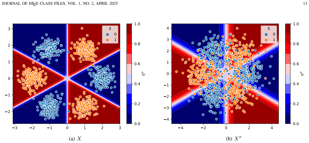
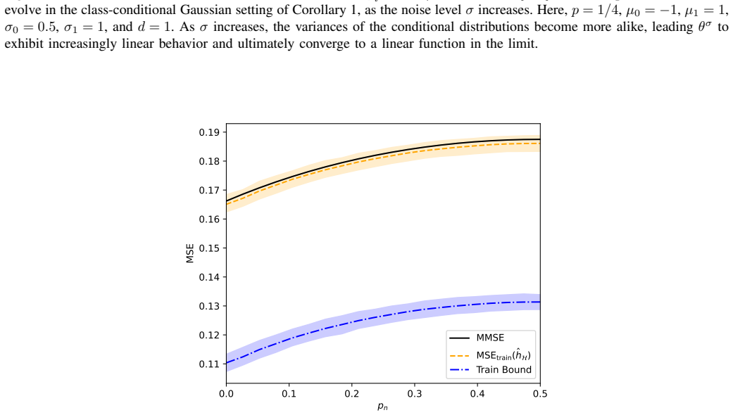
The central result (Theorem 1) is that for every hypothesis class H of functions into [0,1] and sensitive feature S∈[0,1], MMSE(S|Xσ) ≥ MSEtrain(ĥH) − ϵC − ϵA, where MSEtrain(ĥH) is the training mean-squared error of the empirical risk minimizer, ϵC is a concentration term controlled by standard large-deviation bounds on bounded losses, and ϵA = ∥ησ − h*_H∥² is the population gap between the best-in-class predictor and the true conditional expectation. The proof splits the gap into a finite-sample term and an approximation term, and a companion validation-based bound (Theorem 2) replaces part of the training error with validation error at the cost of a generalization term. For linear models under the sigmoid link, ϵA is bounded in closed form through a variance decomposition of the optimal logit θσ(Xσ), giving ϵA=0 for linear or equal-covariance Gaussian relationships, O(1/σ²) decay for the binary symmetric channel, and O(1/σ⁴) decay for class-conditional Gaussians with unequal covariances, where the bound grows quadratically with dimension. The message is that a simple finite-capacity linear model run by a red team yields non-vacuous guarantees on the strongest adversary, provided the noise level is not too small.
Load-bearing premise
The red team must be able to obtain the population-level quantities ϵA and the variance of the squared-loss variable, or have them be negligible; in practice these require either knowing the true data-generating distribution or using very large auxiliary samples, so the advertised finite-sample bound is not directly computable from the n training pairs alone.
Editorial extensions
If this is right
- For binary S, the MMSE lower bound transfers to a lower bound on the probability of misclassification, so the framework certifies a floor on adversarial accuracy, not just on squared error.
- When S is a linear function of X or the classes share a covariance matrix, ϵA = 0 and the only gap is the concentration term, which shrinks as n grows; the training bound then becomes an arbitrarily tight audit of the noise mechanism.
- For the binary symmetric channel and unequal-covariance Gaussian classes, the closed-form approximation bounds decay at rate O(1/σ²) and O(1/σ⁴) respectively, so at large noise a linear red-team model estimates the true MMSE almost exactly.
- The validation-based bound allows richer hypothesis classes such as neural networks, but the experiments show the compression-based generalization bound is vacuous at realistic sizes, so the training-based bound is currently the practically reliable one.
Reading between the lines
- Beyond the paper, the same decomposition should hold for any additive noise mechanism, not just Gaussian, since it relies only on boundedness of S and of the hypothesis outputs; re-deriving the concentration term for other noise distributions would extend the audit framework without new conceptual machinery.
- The quadratic growth of the linear-model approximation error in dimension suggests a practical design rule: for high-dimensional releases, either raise the noise level σ, increase the evaluation sample size, or switch to a neural network class whose approximation error is negligible once overfitting is controlled.
- A direct testable extension is to run the training bound on a real dataset using only the n labeled pairs to estimate every term—without the paper's 1M auxiliary samples—and compare against a high-fidelity Monte Carlo MMSE; the paper's synthetic results predict the bound stays non-negative and tight for moderate n.
- If a non-vacuous generalization bound for square loss were found, the validation bound (Theorem 2) would become the preferred audit tool; the paper's negative finding indicates that the coding-length complexity term, not the framework, is the current bottleneck.
Signed reviews
Editorial analysis
A structured set of objections, weighed in public.
Referee Report
Summary. The paper proposes a framework for lower-bounding the minimum mean-squared error (MMSE) with which a sensitive attribute S in [0,1] can be inferred from a noisy release Xσ = X + σZ, using a finite sample of (Xσ,S) pairs and a restricted hypothesis class H. The central result (Theorem 1) decomposes the gap between the empirical training MSE of an ERM ĥH and the true MMSE into a concentration term ϵC and an approximation term ϵA = ||ησ - h*H||², yielding MMSE ≥ MSEtrain(ĥH) - ϵC - ϵA. A second result (Theorem 2) attempts the same with the validation MSE, at the cost of an additional generalization term ϵG controlled by a compression-based bound. For sigmoid-composed-with-linear models, the paper derives closed-form bounds on ϵA for several generative models (binary symmetric channel, equal- and unequal-covariance class-conditional Gaussians), including noise-rate and dimension dependence. Experiments on BSC, CCG, and Gaussian-mixture data compare linear and neural-network evaluators, document that validation-based bounds are vacuous in practice, and show that the analytic ϵA bounds are loose for small σ. The paper explicitly acknowledges several limitations, including the population-level nature of ϵA and the looseness of the analytic bounds.
Significance. If the results held as written, this would be a useful, inexpensive privacy-auditing tool: it converts the training or validation MSE of a simple model into a finite-sample lower bound on the inference power of an unrestricted adversary, with closed-form approximation-error bounds for several important generative models. Genuine strengths: Theorem 1 is correct and its proof is clean, relying on a clever pointwise decomposition that avoids generalization bounds; the closed-form approximation-error bounds for class-conditional Gaussians (Theorem 4, Corollary 1) are substantial and appear correct, including the explicit dimension dependence; and the empirical evaluation is unusually honest, reporting the vacuousness of the compression-based validation bounds, the looseness of the analytic bounds at small σ, and the overfitting of neural networks. However, the new validation-based claim (Theorem 2) is not proven as written because of a sign error, and the BSC bound (Theorem 3) is a formal asymptotic rather than a rigorous theorem.
major comments (3)
- [Section III, Theorem 2 / Eq. (22) and Appendix B, Eq. (71)] The proof of the validation lower bound has a sign inconsistency that invalidates the theorem as stated. Equation (22) defines ϵG := MSEtrain(ĥH) - E[(S - ĥH)²], but in the chain in Eq. (71) the proof substitutes E[(S - ĥH)²] - MSEtrain(ĥH) = ϵG; the correct identity is E[(S - ĥH)²] - MSEtrain(ĥH) = -ϵG. The resulting correct chain is I ≤ ϵC - ϵG, so Δval ≤ ϵ̃C + ϵC - ϵG + ϵA and hence MMSE ≥ MSEval - ϵ̃C - ϵC + ϵG - ϵA. The claimed inequality (20) follows only when ϵG ≥ 0; in the overfitting regime ϵG < 0, which is precisely the regime the validation bound is introduced to address, the claimed bound is stronger than what the proof establishes. Proposition 2 compounds the problem: it states a high-probability upper bound on ϵG under the definition (22), but the proof requires an upper bound on -ϵG (equivalently, on E[(S - ĥH)²] - MSEtrain(ĥH)); a compression bound of the type quoted in (24) controls the population-minus-training gap in the opposite direction and is vacuous for the needed quantity when ϵG < 0. The error appears repairable by redefining ϵG with the opposite sign, which also matches the conventional meaning of 'generalization error' used in Remark 3, and then restating Theorem 2, Proposition 2, and the related discussion consistently.
- [Section IV, Theorem 3, Eq. (33)] The stated bound on ϵA for the BSC is not a proven inequality for any fixed σ. Expression (33) contains two O(·) remainder terms with unspecified constants C1(p,pN) and C2(p,pN), and Appendix D computes only the first few terms of formal power-series expansions, with no justification of termwise integration of the series in (86) and (104), no convergence radius, and no explicit remainder estimate. As written, (33) is a formal asymptotic expansion, and a reader cannot verify that ϵA ≤ ϵABSC for any particular value of σ. Since the abstract and the contribution list advertise closed-form bounds for binary symmetric channels, the authors should either derive explicit bounds with computable constants that hold for all σ (or for a quantified range), or restate Theorem 3 as an asymptotic statement with explicit remainder control. Note also that Figure 3 evaluates only the first four terms of (33), which is not covered by the theorem as it stands; Section IV-A correctly acknowledges loosness at small σ, but that concession does not cure the formal gap in the theorem statement.
- [Section V ('Computability of bounds'), Sections II-III] The advertised finite-sample nature of the lower bounds is only partially realized, as the paper itself acknowledges. The bound in Theorem 1 contains ϵA = ||ησ - h*H||², a population quantity not computable from the n training samples without knowledge of the true conditional expectation ησ; the tighter Bernstein form of Proposition 1 also requires h*H (Remark 2); and Theorem 2 inherits both requirements. In the experiments, ϵA, ησ, and h*H are estimated using 1M samples together with knowledge of the generative model, while only MSEtrain and MSEval are computed from the advertised finite sample. The paragraph 'Computability of bounds' correctly notes that ϵA can be made small by choosing a rich H at the price of more training samples, but the abstract and contribution statements still describe the results as finite-sample lower bounds. I recommend that the paper state precisely which components of (13) and (20) are computable from the n (and m) samples alone, which require distributional knowledge, and under what conditions the bound becomes a fully data-driven guarantee.
minor comments (8)
- [Section I-A] The sentence 'In constrast to these approaches, we problem we consider here differs in two ways' is garbled and should be rewritten.
- [Theorem 4, Eq. (38)] The matrix index 'y' in 'Σ̃1/2 y A Σ̃1/2 y' should be 's' to be consistent with the surrounding notation.
- [Theorem 3 and Appendix D] The notation 'pNpN', 'qq', and 'pNp' is hard to parse; I suggest introducing explicit symbols such as p̄N := 1-pN and q̄ := 1-q throughout the theorem and its proof.
- [Proposition 3, proof] The statement that h*H(x) = s(θ*L(x)) for θ*L minimizing ||θσ - θL||² is not generally true, since minimizing E[(S - s(θL))²] over linear θL need not coincide with s of the linear projection of θσ; the bound (30) remains valid without this equality, but the proof should present (30) as an inequality rather than an equality.
- [Proposition 2] Because the central validation bound relies on [2, Thm. 3.1], a recent preprint, the paper should restate the precise conditions of that theorem and the coding scheme used so that Proposition 2 is self-contained.
- [Manuscript header] The header states 'Manuscript received October 26, 2023; revised December 8, 2023,' which is inconsistent with an April 2025 submission; the dates should be updated.
- [Proposition 1] The phrase 'new Bernstein-style bound' overstates the novelty: the bound is an application of the empirical Bernstein inequality of Maurer and Pontil [34] to the quantity ϵC; the wording should be adjusted.
- [Section V, experimental protocol] The protocol should clarify that the estimates of ησ, h*H, and ϵA are oracle quantities that use knowledge of the generative model, in contrast to MSEtrain and MSEval, which use only the finite sample; this distinction is currently stated only implicitly.
Circularity Check
No circularity found: the MMSE lower bounds follow from direct loss decompositions with explicit concentration and approximation error terms.
full rationale
The paper's central result (Theorem 1) is a self-contained decomposition: by adding and subtracting MMSEH(S|Xσ), the gap between the empirical training MSE and the true MMSE is split into a finite-sample concentration term ϵC and an approximation term ϵA, and each is then bounded (Hoeffding or empirical Bernstein for ϵC; direct L2 approximation analyses for ϵA). No fitted parameter is renamed as a prediction, and the bound is not derived from the quantity it bounds. Theorem 2 is a parallel validation-loss decomposition; the sign error in the proof identified by the reviewer is a correctness issue, not a circular reduction, because the claimed inequality could fail while the decomposition itself remains non-tautological. The heavy self-citation to [1] is provenance: the paper states that prior versions omitted proofs and includes full proofs here, so the arguments do not reduce to an unverified self-citation. The empirical sections use large-sample estimates of population quantities such as ϵA, which the authors explicitly acknowledge as a limitation of practical computability, but that is not a circularity. The authors' own admission that the validation bound is vacuous in Figure 9 and accompanying text further confirms the bounds are not being forced by construction.
Assumptions & free parameters
free parameters (1)
- C1(p, pN) and C2(p, pN) in Theorem 3
assumptions (5)
- standard math MMSE(S|Xσ) is attained by the conditional expectation ησ and MMSE_H(S|Xσ) = ||ησ − h*_H||² + MMSE(S|Xσ) for any h*_H ∈ H.
- standard math The sigmoid function s(z) = 1/(1+e^{-z}) is 1/4-Lipschitz.
- standard math Hoeffding's inequality and the empirical Bernstein inequality of Maurer and Pontil hold for bounded [0,1] random variables.
- domain assumption Wilson's compression-based generalization bound (arXiv:2503.02113, Thm 3.1) provides a valid uniform upper bound on the generalization error of ĥH.
- domain assumption The sanitized data follow Xσ = X + σZ with Z∼N(0,I) independent of (X,S), and X|S follows one of the specified families (BSC, class-conditional Gaussian with equal or unequal covariances, Gaussian mixture).
Cite this review
Pith. "Pith review of Lower Bounds on the MMSE of Adversarially Inferring Sensitive Features." pith.science (2026). https://pith.science/paper/N2EWAA3A
@misc{pith2026250509004,
  author       = {Pith},
  title        = {Pith review of: Lower Bounds on the MMSE of Adversarially Inferring Sensitive Features},
  year         = {2026},
  howpublished = {\url{https://pith.science/paper/N2EWAA3A}},
  note         = {Machine review of arXiv:2505.09004}
}
read the original abstract
We propose an adversarial evaluation framework for sensitive feature inference based on minimum mean-squared error (MMSE) estimation with a finite sample size and linear predictive models. Our approach establishes theoretical lower bounds on the true MMSE of inferring sensitive features from noisy observations of other correlated features. These bounds are expressed in terms of the empirical MMSE under a restricted hypothesis class and a non-negative error term. The error term captures both the estimation error due to finite number of samples and the approximation error from using a restricted hypothesis class. For linear predictive models, we derive closed-form bounds, which are order optimal in terms of the noise variance, on the approximation error for several classes of relationships between the sensitive and non-sensitive features, including linear mappings, binary symmetric channels, and class-conditional multi-variate Gaussian distributions. We also present a new lower bound that relies on the MSE computed on a hold-out validation dataset of the MMSE estimator learned on finite-samples and a restricted hypothesis class. Through empirical evaluation, we demonstrate that our framework serves as an effective tool for MMSE-based adversarial evaluation of sensitive feature inference that balances theoretical guarantees with practical efficiency.
Figures


Figures from the paper (14 more)






Reference graph
Works this paper leans on
-
[1]
Auditing privacy of additive noise mechanisms using linear predictive models,
M. Welfert, N. Stromberg, M. Diaz, J. Melbourne, and L. Sankar, “Auditing privacy of additive noise mechanisms using linear predictive models,” 2025, accepted for presentation at ISIT 2025. [Online]. Available: https://github.com/SankarLab/mmse-estimate-finite-samples-finite-capacity-models/ tree/main/papers
work page 2025
-
[2]
Deep learning is not so mysterious or different,
A. G. Wilson, “Deep learning is not so mysterious or different,” arXiv preprint arXiv:2503.02113 , 2025
arXiv 2025
-
[3]
L. L. Scharf and C. Demeure, Statistical Signal Processing: Detection, Estimation, and Time Series Analysis . Prentice Hall, 1991
1991
-
[4]
E. Biglieri, R. Calderbank, A. Constantinides, A. Goldsmith, A. Paulraj, and H. V . Poor, MIMO Wireless Communications. Cambridge University Press, 2007. JOURNAL OF LATEX CLASS FILES, VOL. 1, NO. 2, APRIL 2025 16
work page 2007
-
[5]
Mutual information and minimum mean-square error in Gaussian channels,
D. Guo, S. Shamai, and S. Verd ´u, “Mutual information and minimum mean-square error in Gaussian channels,” IEEE Transactions on Information Theory, vol. 51, no. 4, pp. 1261–1282, 2005
work page 2005
-
[6]
Estimation in Gaussian noise: Properties of the minimum mean-square error,
D. Guo, Y . Wu, S. S. Shitz, and S. Verd ´u, “Estimation in Gaussian noise: Properties of the minimum mean-square error,” IEEE Transactions on Information Theory, vol. 57, no. 4, pp. 2371–2385, 2011
work page 2011
-
[7]
Functional properties of minimum mean-square error and mutual information,
Y . Wu and S. Verd ´u, “Functional properties of minimum mean-square error and mutual information,” IEEE Transactions on Information Theory , vol. 58, no. 3, pp. 1289–1301, 2011
work page 2011
-
[8]
An mmse lower bound via poincar ´e inequality,
I. Zieder, A. Dytso, and M. Cardone, “An mmse lower bound via poincar ´e inequality,” in 2022 IEEE International Symposium on Information Theory (ISIT), 2022, pp. 957–962
work page 2022
Show all 46 references
-
[9]
The strong data processing inequality under the heat flow,
B. Klartag and O. Ordentlich, “The strong data processing inequality under the heat flow,” IEEE Transactions on Information Theory , pp. 1–1, 2025
2025
-
[10]
A comprehensive study on ziv-zakai lower bounds on the mmse,
M. Jeong, A. Dytso, and M. Cardone, “A comprehensive study on ziv-zakai lower bounds on the mmse,” IEEE Transactions on Information Theory , vol. 71, no. 4, pp. 3214–3236, 2025
2025
-
[11]
A statistical analysis of the kernel-based MMSE estimator with application to image reconstruction,
A. M. Peinado, J. Koloda, A. M. Gomez, and V . Sanchez, “A statistical analysis of the kernel-based MMSE estimator with application to image reconstruction,” Signal Processing: Image Communication , vol. 55, pp. 41–54, 2017
2017
-
[12]
Mutual information as a function of moments,
W. Alghamdi and F. P. Calmon, “Mutual information as a function of moments,” in 2019 IEEE International Symposium on Information Theory (ISIT) . IEEE, 2019, pp. 3122–3126
2019
-
[13]
Polynomial approximations of conditional expectations in scalar Gaussian channels,
——, “Polynomial approximations of conditional expectations in scalar Gaussian channels,” in 2021 IEEE International Symposium on Information Theory (ISIT). IEEE, 2021, pp. 420–425
2021
-
[14]
Measuring information from moments,
——, “Measuring information from moments,” IEEE Transactions on Information Theory , vol. 70, no. 2, pp. 763–802, 2024
2024
-
[15]
The composition theorem for differential privacy,
P. Kairouz, S. Oh, and P. Viswanath, “The composition theorem for differential privacy,” IEEE Transactions on Information Theory , vol. 63, no. 6, pp. 4037–4049, 2017
2017
-
[16]
Operational definitions for some common information leakage metrics,
I. Issa and A. B. Wagner, “Operational definitions for some common information leakage metrics,” in 2017 IEEE International Symposium on Information Theory (ISIT). IEEE, 2017, pp. 769–773
2017
-
[17]
Tunable measures for information leakage and applications to privacy-utility tradeoffs,
J. Liao, O. Kosut, L. Sankar, and F. du Pin Calmon, “Tunable measures for information leakage and applications to privacy-utility tradeoffs,” IEEE Transactions on Information Theory , vol. 65, no. 12, pp. 8043–8066, 2019
2019
-
[18]
Estimation efficiency under privacy constraints,
S. Asoodeh, M. Diaz, F. Alajaji, and T. Linder, “Estimation efficiency under privacy constraints,” IEEE Transactions on Information Theory , vol. 65, no. 3, pp. 1512–1534, 2019
2019
-
[19]
Learning and generalization with the information bottleneck,
O. Shamir, S. Sabato, and N. Tishby, “Learning and generalization with the information bottleneck,” Theoretical Computer Science, vol. 411, no. 29-30, pp. 2696–2711, 2010
2010
-
[20]
Minimax estimation of functionals of discrete distributions,
J. Jiao, K. Venkat, Y . Han, and T. Weissman, “Minimax estimation of functionals of discrete distributions,” IEEE Transactions on Information Theory , vol. 61, no. 5, pp. 2835–2885, 2015
2015
-
[21]
Minimax rates of entropy estimation on large alphabets via best polynomial approximation,
Y . Wu and P. Yang, “Minimax rates of entropy estimation on large alphabets via best polynomial approximation,” IEEE Transactions on Information Theory, vol. 62, no. 6, pp. 3702–3720, 2016
2016
-
[22]
On the robustness of information-theoretic privacy measures and mechanisms,
M. Diaz, H. Wang, F. P. Calmon, and L. Sankar, “On the robustness of information-theoretic privacy measures and mechanisms,” IEEE Transactions on Information Theory, vol. 66, no. 4, pp. 1949–1978, 2019
1949
-
[23]
Mutual information neural estimation,
M. I. Belghazi, A. Baratin, S. Rajeshwar, S. Ozair, Y . Bengio, A. Courville, and D. Hjelm, “Mutual information neural estimation,” in International Conference on Machine Learning . PMLR, 2018, pp. 531–540
2018
-
[24]
Neural entropic estimation: A faster path to mutual information estimation,
C. Chan, A. Al-Bashabsheh, H. P. Huang, M. Lim, D. S. H. Tam, and C. Zhao, “Neural entropic estimation: A faster path to mutual information estimation,” arXiv preprint arXiv:1905.12957 , 2019
1905 arXiv
-
[25]
Non-asymptotic performance guarantees for neural estimation of f-divergences,
S. Sreekumar, Z. Zhang, and Z. Goldfeld, “Non-asymptotic performance guarantees for neural estimation of f-divergences,” in International Conference on Artificial Intelligence and Statistics . PMLR, 2021, pp. 3322–3330
2021
-
[26]
Auditing differentially private machine learning: How private is private sgd?
M. Jagielski, J. Ullman, and A. Oprea, “Auditing differentially private machine learning: How private is private sgd?” Advances in Neural Information Processing Systems, vol. 33, pp. 22 205–22 216, 2020
2020
-
[27]
Adversary instantiation: Lower bounds for differentially private machine learning,
M. Nasr, S. Songi, A. Thakurta, N. Papemoti, and N. Carlin, “Adversary instantiation: Lower bounds for differentially private machine learning,” in 2021 IEEE Symposium on Security and Privacy (SP) . IEEE, 2021, pp. 866–882
2021
-
[28]
Neural network-based estimation of the MMSE,
M. Diaz, P. Kairouz, J. Liao, and L. Sankar, “Neural network-based estimation of the MMSE,” in 2021 IEEE International Symposium on Information Theory (ISIT). IEEE, 2021, pp. 1023–1028
2021
-
[29]
Universal approximation bounds for superpositions of a sigmoidal function,
A. R. Barron, “Universal approximation bounds for superpositions of a sigmoidal function,” IEEE Transactions on Information Theory , vol. 39, no. 3, pp. 930–945, 1993
1993
-
[30]
The algorithmic foundations of differential privacy,
C. Dwork and A. Roth, “The algorithmic foundations of differential privacy,” Found. Trends Theor. Comput. Sci., vol. 9, no. 3-4, pp. 211–407, 2014
2014
-
[31]
Privacy-aware MMSE estimation,
S. Asoodeh, F. Alajaji, and T. Linder, “Privacy-aware MMSE estimation,” in 2016 IEEE International Symposium on Information Theory (ISIT) . IEEE, 2016, pp. 1989–1993
2016
-
[32]
Information extraction under privacy constraints,
S. Asoodeh, M. Diaz, F. Alajaji, and T. Linder, “Information extraction under privacy constraints,” Information, vol. 7, no. 1, p. 15, 2016
2016
-
[33]
Shalev-Shwartz and S
S. Shalev-Shwartz and S. Ben-David, Understanding Machine Learning: From Theory to Algorithms . Cambridge University Press, 2014
2014
-
[34]
Empirical bernstein bounds and sample variance penalization,
A. Maurer and M. Pontil, “Empirical bernstein bounds and sample variance penalization,” in Conference on Learning Theory (COLT) , 2009
2009
-
[35]
Rademacher and gaussian complexities: Risk bounds and structural results,
P. L. Bartlett and S. Mendelson, “Rademacher and gaussian complexities: Risk bounds and structural results,” Journal of Machine Learning Research (JMLR), vol. 3, no. Nov, pp. 463–482, 2002
2002
-
[36]
Adaptive and learning systems for signal processing communications, and control,
V . N. Vapnik, “Adaptive and learning systems for signal processing communications, and control,” Statistical learning theory , 1998
1998
-
[37]
Hastie, R
T. Hastie, R. Tibshirani, and J. Friedman, The elements of statistical learning: data mining, inference and prediction . Springer, 2009
2009
-
[38]
Lower bounds on the mmse of adversarially inferring sensitive features,
M. Welfert, N. Stromberg, M. Diaz, and L. Sankar, “Lower bounds on the mmse of adversarially inferring sensitive features,” https://github.com/ SankarLab/mmse-estimate-finite-samples-finite-capacity-models/, 2025
2025
-
[39]
Pac-bayes compression bounds so tight that they can explain generalization,
S. Lotfi, M. Finzi, S. Kapoor, A. Potapczynski, M. Goldblum, and A. G. Wilson, “Pac-bayes compression bounds so tight that they can explain generalization,” Advances in Neural Information Processing Systems , vol. 35, pp. 31 459–31 473, 2022
2022
-
[40]
Mathai and S
A. Mathai and S. Provost, Quadratic Forms in Random Variables , ser. Statistics: A Series of Textbooks and Monographs. Taylor & Francis, 1992. APPENDIX A. Proof of Theorem 1 For ease of notation, we define ∆train := MSEtrain(ˆhH)− MMSE(S|Xσ). (51) Note that we can rewrite ∆tra...
1992
-
[41]
JOURNAL OF LATEX CLASS FILES, VOL
+q(I02−I2 0), (101) where I02 := E[θσ(Xσ)2|X = 0] = Z ∞ −∞ θσ(σz)2fZ(z)dz, (102) I12 := E[θσ(Xσ)2|X = 1] = Z ∞ −∞ θσ(1 +σz)2fZ(z)dz, (103) and fZ is again the density of the standard Gaussian random variable Z. JOURNAL OF LATEX CLASS FILES, VOL. 1, NO. 2, APRIL 2025 21 Again u...
2025
-
[42]
(120) Finally, we have that Cov(θσ(Xσ),Xσ) = Cov(θσ(Xσ),X ) +σCov(θσ(Xσ),Z ) (121) =qq(I1−I0) +σ (qE[Zθσ(σZ)] +qE[Zθσ(1 +σZ)])
+q(I12−I2 1) ≈ 3(1− 2pN)2 σ2 + (1− 2pN)2(5− 4pN + 4p2 N + 12q) 2σ4 + pNpN(1− 2pN)2 2σ6 − p2 N(1− 3pN + 2p2 N)2 4σ8 . (120) Finally, we have that Cov(θσ(Xσ),Xσ) = Cov(θσ(Xσ),X ) +σCov(θσ(Xσ),Z ) (121) =qq(I1−I0) +σ (qE[Zθσ(σZ)] +qE[Zθσ(1 +σZ)]). (122) JOURNAL OF LATEX CLASS FIL...
2025
-
[43]
+∥µ1∥2 2−∥µ0∥2 2)(µ1−µ0)T +bT αI +p(1−p)(µ1−µ0)(µ1−µ0)T (177) =γ1µT 1 +γ0µT
-
[44]
(178) where α :=pσ2 1 + (1−p)σ2 0 +σ2 (179) and γ1 :=a 2p(σ2 1 +σ2) +p(1−p)(d(σ2 1−σ2
-
[45]
+∥µ1∥2 2−∥µ0∥2 2) + α σ2 1 +σ2 +p(1−p)(σ2 0 +σ2)∥µ1∥2 2−(σ2 1 +σ2 0 + 2σ2)µT 1µ0 + (σ2 1 +σ2)∥µ0∥2 2 (σ2 1 +σ2)(σ2 0 +σ2) , (180) γ0 :=a 2(1−p)(σ2 0 +σ2)−p(1−p)(d(σ2 1−σ2
-
[46]
(181) JOURNAL OF LATEX CLASS FILES, VOL
+∥µ1∥2 2−∥µ0∥2 2) − α σ2 0 +σ2 −p(1−p)(σ2 0 +σ2)∥µ1∥2 2−(σ2 1 +σ2 0 + 2σ2)µT 1µ0 + (σ2 1 +σ2)∥µ0∥2 2 (σ2 1 +σ2)(σ2 0 +σ2) . (181) JOURNAL OF LATEX CLASS FILES, VOL. 1, NO. 2, APRIL 2025 27 Again making the appropriate substitutions, (44) reduces to Var(Xσ) =αI +p(1−p)(µ1−µ0)(µ...
2025
Reviewed August 15, 2026 · model on record in the stance chip above.
Discussion (0). Continue with ORCID to comment.