REVIEW 4 major objections 5 minor 42 references
Wave propagation phenomena in nonlinear hierarchical neural networks with predictive coding feedback dynamics
T0 review · 4 major / 5 minor · reviewed 2026-08-15 · deepseek-v4-flash
Pith's one-line read In a nonlinear predictive-coding network, the direction of activity propagation is controlled by the signs of two unique traveling-wave speeds, and input thresholds separate propagation from stagnation.
desk verdict A genuinely useful nonlinear extension of predictive-coding lattice dynamics with a rigorous bi-infinite wave front analysis, but the semi-infinite sharp thresholds s0* and tau* are numerical observations that the abstract oversells. read the letter →
The pith
A machine-rendered reading of the paper's core claim, the machinery that carries it, and where it could break.
The reading
What carries the argument
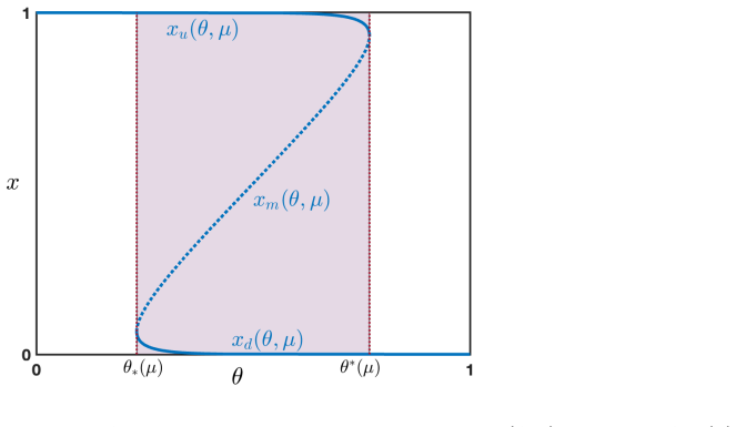
The central machinery is the scalar lattice equation (3.1) with the three-point nonlinearity $N(u,v,w)=(1-p-q)(S(u)-v)+pS'(v)(u-S(v))+q(S(w)-v)$ acting between neighboring layers, where $S(x)=1/(1+e^{-\mu(x-\theta)})$ is the sigmoid activation. On a bi-infinite lattice the equation is bistable in the parameter regime $\mathcal{P}$: the homogeneous stationary states are exactly the down state $x_d$, the unstable middle state $x_m$, and the up state $x_u$, and the dynamics between them is carried by monotone traveling fronts $\Phi_{u\to d}$ and $\Psi_{d\to u}$. A theorem of Mallet-Paret applied to this discrete bistable system supplies existence, uniqueness, and continuous dependence of the front speeds $c_{u\to d}$ and $c_{d\to u}$; the sign of those speeds, rather than their magnitude, is the quantity that determines the long-time behavior. A comparison principle (Lemmas A.1 and A.2) then extends the wave picture to semi-infinite domains and input-driven initiation, where the stationary solutions $x_d(s_0)$ and $x_u(s_0)$ of the boundary-value problems (3.12) and (3.13) serve as the stagnation and propagation targets.
What would settle it
Fix a parameter set in $\mathcal{P}$ with $c_{u\to d}>0$, run the semi-infinite system (3.10)-(3.11) with constant input for amplitudes $s_0$ in a fine grid straddling the reported $s_0^*$, and check the long-time limit; the sharp-threshold claim fails if any $s_0<s_0^*$ yields local uniform convergence to $x_u(s_0)$, or any $s_0>s_0^*$ yields uniform convergence to $x_d(s_0)$.
Extended reading notes
Core claim
The central claim is that, for the one-population model obtained by setting the feedforward and feedback weight matrices to the identity, the propagation properties of the hierarchy are completely described by two monotone traveling fronts and their speeds. For every parameter set in the bistable regime $\mathcal{P}$, there exist a unique decreasing front $\Phi_{u\to d}$ connecting the up state $x_u$ to the down state $x_d$ with speed $c_{u\to d}$, and a unique increasing front $\Psi_{d\to u}$ connecting $x_d$ to $x_u$ with speed $c_{d\to u}$. The sign of $c_{u\to d}$ decides whether an up-state region invades a down-state background, and the sign of $c_{d\to u}$ decides the reverse; when both speeds are zero the wave is pinned and the network cannot transmit activity. On semi-infinite networks, the same front structure produces a threshold: a constant input of amplitude $s_0$ below $s_0^*$ leaves the network in a stagnating state converging to $x_d(s_0)$, while above $s_0^*$ the up state propagates; a flashed input of duration $\tau$ below $\tau^*$ fades back to the down state, while longer flashes produce stacked-interface or front propagation. The speeds obey the symmetry $c_{u\to d}(\theta)=c_{d\to u}(1-\theta)$, so $\theta=1/2$ is the balanced point where both directions behave identically.
Load-bearing premise
The load-bearing premise is that the sharp threshold $s_0^*$ between stagnation and propagation, observed in numerical simulations, is an exact dichotomy rather than a numerical artifact; without that, the semi-infinite propagation claims in Sections 3.2 and 3.3 do not follow.
Editorial extensions
If this is right
- Upward propagation of a sensory input requires $c_{u\to d}>0$: outside that parameter region the up state cannot invade the down state, no matter how strong the input.
- In the pinning regions where $c_{u\to d}=c_{d\to u}=0$, the network exhibits intrinsic propagation failure, so information cannot travel from layer to layer.
- For flashed inputs, the ordering of the two speeds selects the spatial pattern: a front when $c_{d\to u}\le 0<c_{u\to d}$, a stacked interface when $0<c_{d\to u}<c_{u\to d}$, and a traveling pulse whose width grows with flash duration when $0<c_{d\to u}=c_{u\to d}$.
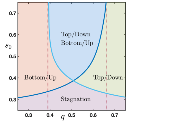
- The amplitude threshold $s_0^*$ diverges as $q$ approaches the value where $c_{u\to d}$ vanishes, so near the pinning boundary even very strong inputs cannot initiate upward propagation.
- The paper postulates that the normal working regime is the parameter region where both bottom-up and top-down propagation coexist ($\theta$ below $1/2$ and intermediate $q$), with the complementary regions corresponding to over-dominance of sensory or endogenous activity.
Reading between the lines
- Editorial inference: the traveling-pulse family at $\theta=1/2$ with width controlled by $\tau$ suggests a concrete coding scheme in which stimulus duration is represented by the spatial extent of a propagating pulse; a rigorous existence proof for this family is left open in the paper.
- Editorial inference: the sharp-threshold dichotomy is a natural target for a theorem; comparison-principle monotonicity in $s_0$ might establish a unique critical amplitude $s_0^*$ at which the stable manifold of $x_u(s_0)$ appears, replacing the current numerical evidence.
- Editorial inference: the symmetry $c_{u\to d}(\theta)=c_{d\to u}(1-\theta)$ hints at an up/down duality that could persist in two-population or asymmetric-weight extensions, where it could be tested by computing front speeds numerically.
- Editorial inference: with the spike-frequency-adaptation term the authors propose, the permanent up state would become transient, and the bistable fronts studied here would be expected to turn into traveling pulses whose existence could be analyzed with the same profile equations augmented by a slow variable.
Signed reviews
Editorial analysis
A structured set of objections, weighed in public.
Referee Report
Summary. The manuscript derives a continuous-time lattice neural-network model motivated by predictive coding, reduces it to the scalar one-population equation (3.1), and analyzes propagation in three settings: bi-infinite networks, semi-infinite networks with constant boundary input, and semi-infinite networks with flashed boundary input. For the bi-infinite bistable regime it claims existence, uniqueness, and monotonicity of traveling fronts by invoking Mallet-Paret's theorem, with wave speeds whose signs are computed numerically over the parameter set P. For the semi-infinite settings it claims that a sharp input-amplitude threshold s0* separates stagnation from upward or downward propagation and that a flashed input has a sharp presentation-time threshold tau*, with the threshold values determined numerically. The paper closes with biological interpretations relating the parameter regions to predictive-coding phenomena and to computational psychiatry.
Significance. If the semi-infinite threshold claims were established, the paper would provide a useful nonlinear extension of the authors' earlier linear analysis [21], with a clean parameter-space classification of bottom-up and top-down propagation and falsifiable predictions about propagation failure. The rigorous parts are genuine strengths: the comparison principles in Lemmas A.1 and A.2 are proved, the parameter regime P is explicit, and the bistable traveling-wave existence is delegated to a verifiable external theorem. However, the central semi-infinite claims--the sharp dichotomy at s0* and tau*--are numerical observations rather than theorems, and the manuscript contains no numerical-convergence evidence supporting their sharpness. The contribution is therefore conditionally significant: the rigorous bi-infinite core is solid, while the semi-infinite propagation results currently outrun their proof.
major comments (4)
- [Section 3.2.1 (Eqs. (3.12)-(3.13))] The sharp threshold dichotomy for s0* is not proved. The text states: "Our numerical investigations ... show the existence of a sharp threshold" and then asserts that for all s0 in [xd(θ,µ),s0*) there is stagnation and for all s0>s0* there is propagation. These two statements require, respectively, existence and uniqueness of the stationary solutions xd(s0) and xu(s0) in (3.12)-(3.13), and actual convergence of the trajectory to one of them. The comparison principle in Lemma A.2 only yields the a priori interval bound vj(t) in [xd,xm] for s0 in [xd,xm]; it does not establish convergence to xd(s0), nor does it rule out alternative asymptotic states. Near the threshold the associated bi-infinite wave speed tends to zero, so any finite-time simulation can misclassify a very slow front as stagnation; the manuscript reports no time horizon, domain truncation, or convergence criterion. Since the abstract promises to "precisely determine" the propagation conditions, this gap is load-bearing.
- [Sections 3.2.2 and 3.3.2] The flashed-input threshold tau* is only "numerically computed"; there is no theorem asserting that the boundary between propagation failure and propagation is sharp. The classification into propagation failure, stacked interface, and front propagation is made from the sign ordering of cu→d and cd→u, but no proof is given that these sign conditions are sufficient for the stated convergence statements on the semi-infinite domain. The critical equal-speed case 0<cd→u=cu→d is explicitly left for future work ("The proper mathematical study of such special solution is beyond the scope of the present study"), yet the abstract and discussion present the flashed-input threshold as part of the precisely determined propagation conditions. The numerical threshold curves in Figures 11 and 16 therefore carry more weight than the text acknowledges.
- [Section 3.3.1] The top-down semi-infinite analysis replicates the same gap for the constant-input threshold. The statement that propagation requires cd→u<0 is a necessary condition imported from the bi-infinite traveling-wave picture; the manuscript does not prove that this condition, together with s0>s0*, implies convergence of the semi-infinite trajectory to the stationary solution yu(s0) in (3.17). The definitions of stagnation and propagation in this subsection also assume without proof the existence and uniqueness of the stationary solutions yd(s0) and yu(s0). Since the top-down results are presented as a complement to the bottom-up analysis and feed into the biological interpretations in Section 3.4, the missing convergence proof is not merely cosmetic.
- [Figures 7, 8, 11, 13, 16] The numerical evidence for the thresholds is not verifiable as reported. The manuscript specifies parameter values (µ=16, p=0.1 and selected q,θ) but gives no discretization of (3.10), no time-stepping scheme, no domain size, no tolerances, and no criterion for deciding that a solution has converged to a stationary state versus propagating with a very small speed. Because the sharpness of s0* and tau* is the central novel claim for the semi-infinite model, the authors should either provide a reproducible numerical protocol with convergence checks or reformulate the statements as numerical observations rather than exact thresholds.
minor comments (5)
- [Section 3.1.3] The invocation of Mallet-Paret's theorem in [28] should be made checkable by stating the precise theorem and explicitly verifying its hypotheses. The manuscript checks ∂uN>0 and ∂wN>0 and the bistable structure of Fp, but the reader is left to infer that these are the exact conditions required by the cited result.
- [Eqs. (3.16)-(3.17)] In the top-down stationary equations the limit condition "yj → j→+∞ xd(θ,µ)" should read j→−∞; the sequence is indexed over j≤−1, so the far-field limit is at −∞. This appears twice and is a mathematical typo that should be corrected.
- [Section 3.2.1 and 3.3.1] The initial conditions in (3.11) and (3.15) write vj(0)=ud(θ,µ), but the stable stationary states constructed in Section 3.1.1 are denoted xd(θ,µ) and xu(θ,µ). The notation should be unified.
- [Appendix A, Lemma A.1 proof] Several lines in the proof of Lemma A.1 contain malformed expressions, e.g. "p(S′(vℓ(t))−S′(wℓ(Tϵ))wℓ−1(Tϵ)" has mismatched parentheses and a stray t, and a similar expression appears later. These should be rewritten as p(S′(vℓ(Tϵ))−S′(wℓ(Tϵ)))wℓ−1(Tϵ) or the intended equivalent. As written, this part of the proof cannot be parsed unambiguously.
- [Sections 3.2.1 and 3.3.1] The symbol q0 is used with different meanings in the bottom-up case (smallest q with cu→d=0) and the top-down case (largest q with cd→u=0). This overloaded notation is confusing when Figures 7 and 13 are compared; distinct symbols would improve clarity.
Circularity Check
No circularity found: wave-front results come from external theorems, and the semi-infinite thresholds are explicitly numerical observations, not fitted inputs relabeled as predictions.
full rationale
Walking the derivation chain, I find no step that reduces a claimed result to its inputs by construction. The nonlinear model (3.1) is obtained by an explicit formal continuous-time limit from the recurrence (2.1), with the sigmoid and the time-rescaling parameters p, q stated in the text; wave-front existence and uniqueness are delegated to Mallet-Paret [28], convergence to the wave is delegated to [12,42], and the comparison principles used for the semi-infinite analysis are proved in Lemmas A.1-A.2. The semi-infinite thresholds s0* and tau* are not presented as derived predictions: the paper states 'Our numerical investigations (see Figures 7 and 8) show the existence of a sharp threshold' and says the flashed threshold was 'numerically computed,' so these are numerical observations rather than fitted parameters renamed as predictions. The only self-reference to the authors' earlier linear model [21] is motivational and methodological ('Proceeding similarly as in [21]'); it does not supply the bistable wave-speed, existence, or threshold claims, which rest on external theorems and the paper's own lemmas. The unproved sharpness of the numerical stagnation/propagation dichotomy is a rigor limitation, not circularity.
Assumptions & free parameters
assumptions (6)
- standard math Mallet-Paret's theorem [28] guarantees existence, uniqueness, and continuous dependence of monotone bistable lattice traveling waves for every parameter set Lambda in P.
- standard math Chen-Guo-Wu [12] and Zinner [42] guarantee exponential convergence of step-like initial data to the traveling waves when the wave speed is nonzero.
- domain assumption The sigmoid activation with mu>4 and theta in (theta*, theta*) yields exactly three homogeneous stationary states xd, xm, xu, with xd and xu stable and xm unstable.
- domain assumption The model reduces to a scalar one-population system by setting Wf=Wb=Id, so each layer node connects only to the corresponding node in adjacent layers.
- domain assumption The stationary solutions xd(s0) and xu(s0) of (3.12) and (3.13) exist and serve as the convergence targets defining stagnation and propagation.
- domain assumption The signs of the numerically computed wave speeds c_{u->d} and c_{d->u} are treated as exact when constructing the phase diagrams in Figures 4 and 5 and the thresholds s0* and tau*.
Cite this review
Pith. "Pith review of Wave propagation phenomena in nonlinear hierarchical neural networks with predictive coding feedback dynamics." pith.science (2026). https://pith.science/paper/ZPLEJ5UW
@misc{pith2026250509199,
  author       = {Pith},
  title        = {Pith review of: Wave propagation phenomena in nonlinear hierarchical neural networks with predictive coding feedback dynamics},
  year         = {2026},
  howpublished = {\url{https://pith.science/paper/ZPLEJ5UW}},
  note         = {Machine review of arXiv:2505.09199}
}
read the original abstract
We propose a mathematical framework to systematically explore the propagation properties of a class of continuous in time nonlinear neural network models comprising a hierarchy of processing areas, mutually connected according to the principles of predictive coding. We precisely determine the conditions under which upward propagation, downward propagation or even propagation failure can occur in both bi-infinite and semi-infinite idealizations of the model. We also study the long-time behavior of the system when either a fixed external input is constantly presented at the first layer of the network or when this external input consists in the presentation of constant input with large amplitude for a fixed time window followed by a reset to a down state of the network for all later times. In both cases, we numerically demonstrate the existence of threshold behavior for the amplitude of the external input characterizing whether or not a full propagation within the network can occur. Our theoretical results are consistent with predictive coding theories and allow us to identify regions of parameters that could be associated with dysfunctional perceptions.
Figures


Figures from the paper (13 more)




Reference graph
Works this paper leans on
-
[21]
G. Faye, G. Fouilh´ e and R. VanRullen. Mathematical derivation of wave propagation properties in hierarchical neural networks with predictive coding feedback dynamics. Bulletin of Mathematical Biology, vol 85, no 80 (2023) , pp. 1-75
work page 2023
-
[1]
L. Aitchison and M. Lengyel. With or without you: predictive coding and Bayesian inference in the brain. Current opinion in neurobiology , 46, 219-227. (2017)
work page 2017
- [2]
- [3]
-
[4]
A. Alamia and R. VanRullen. Alpha oscillations and traveling waves: Signatures of predictive coding? PLoS Biology, 17.10 (2019): e3000487
work page 2019
-
[5]
E. Bart, S. Bao, D. Holcman. Modeling the spontaneous activity of the auditory cortex. J. Comput. Neurosci. 19 (3) (2005) 357–378
work page 2005
-
[6]
J. Benda and A.V.M Herz. A universal model for spike-frequency adaptation. Neural Comput. 15(11), 2523–2564 (2003)
work page 2003
-
[7]
M Bertalmio, A. Gomez-Villa, A. Martin, J. Vazquez-Corral, D. Kane and J. Malo. Evidence for the intrinsically nonlinear nature of receptive fields in vision Scientific reports, (2020), 10(1), 16277
work page 2020
Show all 42 references
-
[8]
Bowman, D.J
H. Bowman, D.J. Collins, A.K. Nayak and D. Cruse. Is predictive coding falsifiable? Neuroscience and Biobehavioral Reviews, 154, 105404. (2023)
2023
-
[9]
J. Bullier. Feedback connections and conscious vision. Trends in cognitive sciences (2001), vol 5 (9), pp 369-370
2001
-
[10]
Bullier, J.-M
J. Bullier, J.-M. Hup´ e, A.C. James and P. Girard. The role of feedback connections in shaping the responses of visual cortical neurons. Progress in brain research (2001), 134, 193-204
2001
-
[11]
Chalasani and J.C
R. Chalasani and J.C. Principe. Deep predictive coding networks. arXiv preprint, arXiv:1301.3541 (2013)
2013 arXiv
-
[12]
Chen, J-S Guo, and C-C Wu
X. Chen, J-S Guo, and C-C Wu. Traveling waves in discrete periodic media for bistable dynamics. Archive for Rational Mechanics and Analysis 189 (2008): 189-236
2008
-
[13]
Choksi, M
B. Choksi, M. Mozafari, C. Biggs O’May, B. Ador, A. Alamia and R. VanRullen. Predify: Augmenting deep neural networks with brain-inspired predictive coding dynamics Advances in Neural Information Processing Systems, 34, 14069-14083
-
[14]
Corlett, G
P.R. Corlett, G. Horga, P.C. Fletcher, B. Alderson-Day, K. Schmack, and A.R. Powers. Hallucinations and strong priors. Trends in cognitive sciences. 23(2), (2019) 114-127
2019
-
[15]
Dehaene, L
S. Dehaene, L. Charles, J.R. King and S. Marti. Toward a computational theory of conscious process- ing. Current opinion in neurobiology 25, (2014), 76-84. 30
2014
-
[16]
Egner and C
T. Egner and C. Summerfield. Grounding predictive coding models in empirical neuroscience research. Behavioral and Brain Sciences , 36.3 (2013): 210-211
2013
-
[17]
Ermentrout, S.E
G.B. Ermentrout, S.E. Folias and Z. P. Kilpatrick. Spatiotemporal pattern formation in neural fields with linear adaptation. Neural Fields: Theory and Applications (2014): 119-151
2014
-
[18]
Erneux and G
T. Erneux and G. Nicolis. Propagating Waves in Discrete Bistable Reaction-Diffusion Systems.Physica D 67, (1993) 237-244
1993
-
[19]
Felleman D.C
D.J. Felleman D.C. and Van Essen. Distributed hierarchical processing in the primate cerebral cortex. Cerebral cortex, (1991), vol 1 (1), pp 1-47
1991
-
[20]
G. Fath. Propagation Failure of Traveling Waves in a Discrete Bistable Medium. Physica D 116, (1998),176-190
1998
-
[22]
Faye and A
G. Faye and A. Scheel. Existence of pulses in excitable media with nonlocal coupling. Advances in Mathematics, vol 270 (2015), pp. 400-456
2015
-
[23]
C.D Gilbert and W. Li. Top-down influences on visual processing. Nature reviews neuroscience, vol 14, 5 (2013), pp. 350-363
2013
-
[24]
Huang and R.P.N
Y. Huang and R.P.N. Rao. Predictive coding. Wiley Interdisciplinary Reviews: Cognitive Science , 580-593. (2011)
2011
-
[25]
J. P. Keener. Propagation and its Failure in Coupled Systems of Discrete Excitable Cells. SIAM J. Appl. Math. 47, (1987), 556-572
1987
-
[26]
LeCun, K
Y. LeCun, K. Kavukcuoglu and C. Farabet. Convolutional networks and applications in vision. In Proceedings of 2010 IEEE international symposium on circuits and systems , (2010), (pp. 253-256). IEEE
2010
-
[27]
Lotter, G
W. Lotter, G. Kreiman and D. Cox. Deep predictive coding networks for video prediction and unsu- pervised learning. arXiv preprint, arXiv:1605.08104 (2016)
2016 arXiv
-
[28]
Mallet-Paret
J. Mallet-Paret. The global structure of traveling waves in spatially discrete dynamical systems. Journal of Dynamics and Differential Equations , 11 (1999): 49-127
1999
-
[29]
A. C. Marreiros, J. Daunizeau, S.J. Kiebel and K.J. Friston. Population dynamics: variance and the sigmoid activation function. Neuroimage, 42(1), (2008) 147-157
2008
-
[30]
McMains and S
S. McMains and S. Kastner. Interactions of top-down and bottom-up mechanisms in human visual cortex. Journal of Neuroscience, 31 (2011): 587-597
2011
-
[31]
Montague, R.J
P.R. Montague, R.J. Dolan, K.J. Friston and P. Dayan. Computational psychiatry.Trends in cognitive sciences. (2012), 16(1), 72-80. 31
2012
-
[32]
P. Nunez. The brain wave equation: a model for the EEG. Math. Biosci. 21, (1974) 279
1974
-
[33]
D. J. Pinto and G. B. Ermentrout. Spatially structured activity in synaptically coupled neuronal networks: I. Traveling fronts and pulses. SIAM J. Appl. Math. , 62 (2001), pp. 206–225
2001
-
[34]
Rao and D
R.P. Rao and D. H. Ballard. Predictive coding in the visual cortex: a functional interpretation of some extra-classical receptive-field effects. Nature neuroscience (1999) vol 2 (1), pp 79-87
1999
-
[35]
CB Schwenk and A
J. CB Schwenk and A. Alamia. A hierarchical multiscale model of forward and backward alpha-band traveling waves in the visual system. bioRxiv, 024.11. 15.623743 (2024)
2024
-
[36]
S. Shipp. Neural elements for predictive coding. Frontiers in psychology, 7 (2016): 1792
2016
-
[37]
Tarasi, J
L. Tarasi, J. Trajkovic, S. Diciotti, G. di Pellegrino, F. Ferri, M. Ursino, V. Romei. Predictive waves in the autism-schizophrenia continuum: a novel biobehavioral model. Neuroscience et Biobehavioral Reviews (2022) 132, 1-22
2022
-
[38]
Tsodyks, K
M. Tsodyks, K. Pawelzik and H. Markram. Neural networks with dynamic synapses. Neural Comput. 10 (4) (1998) 821–835
1998
-
[39]
Van de Cruys, K
S. Van de Cruys, K. Evers, R. Van der Hallen, L. Van Eylen, B. Boets, L. De-Wit and J. Wagemans. Precise minds in uncertain worlds: predictive coding in autism. Psychological review. 121(4), (2014) 649
2014
-
[40]
Wilson and J.D
H.R. Wilson and J.D. Cowan. Excitatory and inhibitory interactions in localized populations of model neurons. Biophys. J. 12, (1972), 1-24
1972
-
[41]
van Rossum
L.C York and M.C.W. van Rossum. Recurrent networks with short term synaptic depression. J Comput. Neurosci., 27, pages 607–620, (2009)
2009
-
[42]
B. Zinner. Stability of Traveling Wavefronts for the Discrete Nagumo Equation. SIAM J. Math. Anal. 22, (1991), 1016-1020. 32
1991
Reviewed August 15, 2026 · model on record in the stance chip above.
Discussion (0). Continue with ORCID to comment.