REVIEW 4 major objections 4 minor 82 references
Mollifier Layers: Enabling Efficient High-Order Derivatives in Inverse PDE Learning
T0 review · 4 major / 4 minor · reviewed 2026-08-15 · deepseek-v4-flash
Pith's one-line read Mollifier layers replace recursive automatic differentiation in physics-informed networks, producing stable high-order derivatives and better parameter recovery at 6–10× lower memory and time.
desk verdict Mollifier layers as a derivative-computation module are a genuinely useful idea for inverse PDE learning, but the convergence guarantee is overstated and the benchmarks need error bars; still worth serious review. read the letter →
The pith
A machine-rendered reading of the paper's core claim, the machinery that carries it, and where it could break.
The reading
What carries the argument
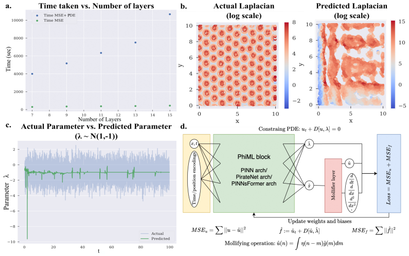
The load-bearing object is the Mollifier Layer: a fixed kernel $\eta$ that is infinitely differentiable, compactly supported, and nonnegative—typically a polynomial or sine bump inside a radius $R$—with the predicted field computed as $\hat{u} = \hat{g} * \eta$ and its derivatives as convolutions with the analytic derivatives of $\eta$. Because $\eta$ and its derivatives are known in closed form and vanish outside a small support, the convolution acts as a localized weak-form integration, the same idea that underlies finite-element test functions and Savitzky-Golay filters. The layer's guarantee is the uniform derivative-consistency bound of Eq. (7): for a $C^1$, $L$-Lipschitz field with bounded pointwise noise, the mollified derivative error is at most $C_1\delta + C_2(h+\varepsilon)$, and choosing $\delta \approx \sqrt{h}$ balances bias against noise. This turns differentiation from an operation whose cost grows with network depth into a single output-layer convolution whose cost is fixed by kernel size.
What would settle it
Take any benchmark from Table 2—say the reaction-diffusion system—and replace the smooth target $\lambda(x,y)$ with one containing a sharp step or oscillation at a spatial frequency above the kernel passband, keeping the noise fixed. The Eq. (7) bound predicts recovery error should rise with kernel width, so a sweep over kernel sizes should show accuracy degrading as $\delta$ grows; if mollified inference instead holds its accuracy at all widths, the proposed error model is wrong.
Extended reading notes
Core claim
The central discovery is that for inverse PDE learning, the derivative oracle matters more than the network. On a trained output $\hat{g}$, the Mollifier Layer forms $\hat{u} = \hat{g} * \eta$ and obtains derivatives such as $\hat{u}_j = \hat{g} * \eta_j$ and $\hat{u}_{jjj} = \hat{g} * \eta_{jjj}$, so all derivatives needed by the PDE residual come from fixed analytic kernels rather than recursive backpropagation through the network. The paper proves, as Eq. (7), that for a $C^1$, $L$-Lipschitz field with bounded pointwise noise, the mollified derivative approximates the true derivative uniformly up to $C_1\delta + C_2(h+\varepsilon)$, so the kernel width $\delta$ can be chosen to balance smoothing bias against noise. In the fourth-order reaction-diffusion benchmark, mollified PINNs raise the spatial correlation of the recovered reaction rate from 0.17 to 0.84 and mollified PirateNet from 0.25 to 0.91, while reducing peak memory from 2.75 GB to 0.23 GB for PINNs. The same layer is then used to infer spatially varying epigenetic reaction rates from super-resolution chromatin images, connecting the numerical method to an interpretable biophysical parameter.
Load-bearing premise
The whole guarantee starts from a smooth-field assumption: the true field is $C^1$ and $L$-Lipschitz, and each noisy sample is bounded by $\varepsilon$; if the true parameter or field varies on a scale finer than the kernel width $\delta$, the smoothing that stabilizes the derivative also blurs away the variation needed for recovery.
Editorial extensions
If this is right
- Attaching a mollifier layer to an existing physics-informed network should immediately reduce the memory and time cost of PDE-residual training; the paper reports 6–10× reductions in time and memory on its benchmarks.
- Networks trained with mollifier layers should recover spatially or temporally varying parameters that recursive autodiff misses; the paper reports spatial-correlation jumps from 0.17 to 0.84 and from 0.25 to 0.91 on the fourth-order reaction-diffusion task.
- High-order derivatives, up to fourth order, become stable under noise, so noisy inverse problems no longer require attention-heavy architectures; a simple mollified PINN outperforms the attention-based PINNsFormer on the tested tasks.
- The same layer should transfer to forward PDE solvers, operator learning, and neural ODEs because derivative computation is detached from network depth; the paper demonstrates a forward toy problem in the appendix.
- The method enables physically interpretable parameters from imaging data: in the application, spatially varying epigenetic reaction rates are inferred from super-resolution chromatin images and match ground-truth domain structure and noise statistics.
Reading between the lines
- The fixed-kernel design suggests that any network output with bounded error can be differentiated stably by convolution, so the practical bottleneck for high-order physics-informed learning may shift from the network to kernel design; adaptive, boundary-aware, or multiscale kernels are natural follow-ups that the paper lists as future work.
- The separable estimator $\hat{\lambda} = \hat{u}_t / D[\hat{u}]$ divides by a learned derivative, and wherever that derivative is near zero the estimate will amplify noise; probing recovery near zero-crossings of $D[\hat{u}]$ would test whether the improvement persists in that regime.
- If the reported efficiency gains generalize, they extend to any convolutional derivative approximation, but the non-negativity and compact-support properties of the mollifier are likely what prevent cancellation errors, so learned kernels that drop those properties may not retain the same noise robustness.
Signed reviews
Editorial analysis
A structured set of objections, weighed in public.
Referee Report
Summary. The paper proposes Mollifier Layers, a module that replaces recursive automatic differentiation in physics-informed machine learning by computing derivatives as convolutions with analytic derivatives of smooth, compactly supported mollifier kernels. The authors test the module on inverse problems for first-, second-, and fourth-order systems (Langevin, heat, reaction-diffusion) across three base architectures (PINN, PirateNet, PINNsFormer) and on a real super-resolution chromatin imaging task, reporting large training-time and memory savings and improved parameter-recovery correlations in most comparisons. The paper also states a uniform convergence guarantee for the mollified derivative estimator in Eq. (7) and derives supporting bounds in Appendix A.8.
Significance. If the reported results hold, the paper would make a useful, architecture-agnostic contribution to inverse PDE learning, addressing a real bottleneck of recursive autodiff. The strengths are the simplicity of the proposed layer, the breadth of comparisons (three architectures and PDE orders up to four), the clear memory/time wins, and the demonstration on a genuinely noisy imaging application. However, the theoretical convergence guarantee appears to be stated with the wrong noise scaling, the empirical tables lack uncertainty estimates, and there is at least one internal contradiction about whether a mollified PINNsFormer was actually evaluated. These issues currently prevent the paper from fully establishing its central claims.
major comments (4)
- [Sec. 3.2, Eq. (7); Appendix A.8, Eqs. (43)-(46)] The stated uniform derivative-consistency bound is not what discrete mollification actually yields. For the mollified finite-difference derivative D0(J_delta g), the noise contribution is (D0 J_delta n)_j = (1/(2h)) * integral of [rho_delta((j+1)h - y) - rho_delta((j-1)h - y)] n(y) dy, and the induced operator norm is O(||rho_delta'||_1) = O(1/delta); for n-th order derivatives the analogous factor is O(delta^{-n}). Equation (43) should therefore read C(delta + h^2 + epsilon/delta), and Eq. (45) should read C_n(delta + h + epsilon/delta^n), not C(delta + h^2 + epsilon). The appendix's own statement that the backward operator norm remains O(1/delta) is incompatible with the bound it quotes. With the recommended choice delta approximately sqrt(h), the noise term becomes epsilon/sqrt(h), so the claimed O(sqrt(h)) uniform consistency and the statement in Sec. 3.2 of 'provably bounded error under discretization and measurement noise' are not established as written. The empirical noise robustness may still be real, but it needs a corrected theoretical analysis or a different justification.
- [Table 2 and Sec. 4.1.1] The text states that Langevin experiments were repeated over five runs per noise level, but Table 2 reports single point values for all correlations, times, and memory figures, with no error bars, standard deviations, or significance tests. Without such uncertainty information, the claimed consistent improvements are not fully supported, especially where the mollified version is numerically worse than its native counterpart (e.g., Langevin PINN mean correlation 0.99 vs. PINN+M 0.96, and temporal correlation 0.99 vs. 0.97; temporal correlation 0.98 vs. 0.97 for PirateNet vs. PirateNet+M). The authors should report run-to-run variability and explain any cases where the mollified model underperforms.
- [Sec. 3.3] The proposed algebraic estimator lambda_final = u_t / D[u] makes the PDE residual in Eq. (3) vanish identically when the governing equation has the form u_t - lambda D[u] = 0. The paper does not say whether the parameter-recovery numbers in Table 2 are obtained from this algebraic rule or by optimizing a network output for lambda against the PDE residual. If the former, the reported 'PDE constraint' results are not an independent test of the mollifier layer's role in enforcing physics, and the residual loss is trivially satisfied; if the latter, the relationship between Eq. (3) and lambda_final must be specified. This distinction is load-bearing for the paper's claim that the method improves parameter recovery through physics-constrained learning.
- [Sec. 4 and Sec. 4.1.1] There is an internal contradiction about whether a mollified PINNsFormer was evaluated. Section 4 states 'we do not include a mollified PINNsFormer' due to computational cost, but Section 4.1.1 says that 'mollified versions surpass native architectures' for PINNsFormer and refers to Figs. 8-10; Table 2 contains no PINNsFormer+M row, and the PINNsFormer appendix figure (Fig. 10) does not show a mollified variant. This contradiction weakens the 'architecture-agnostic across three architectures' claim and should be resolved by explicit reporting of which models were actually run.
minor comments (4)
- [Sec. B.1.2] The sentence 'we also text the models on temporally varying signal' should read 'we also test the models'.
- [Sec. 4.1.1] The phrase 'using a original mollifying function' should be 'using an original mollifying function'.
- [Appendix A.5, Eq. (24)] The exponential mollifier is written as e^{-1/(1-x^2)} in one dimension, but the stated domain is the ball B_R(0); please clarify the variable convention and the normalization constant so that the kernel integrates to unity.
- [Appendix B.5] The forward toy problem is a useful sanity check, but no quantitative result is reported; a short accuracy or error metric would strengthen the claim of applicability beyond inverse problems.
Circularity Check
No significant circularity: the central derivative estimates are benchmarked against external ground truth and the convergence guarantee is imported from an external, non-author theory.
full rationale
The paper's load-bearing comparison (Table 2) is an ablation against external benchmarks with known ground truth: Langevin, heat, and reaction-diffusion systems are simulated, and mollified variants are compared to native PINN/PirateNet/PINNsFormer. No parameter needed for the headline result is fitted to the target derivatives and then renamed a prediction. The derivative estimator is a fixed convolution with analytic mollifier kernels; kernel widths are hand-set per PDE (Appendix A.5) and ablated, not fit to the evaluation data. The convergence guarantee (Eq. 7, Appendix A.8) is explicitly cited to an external, non-author source (Murio et al. 1998) rather than to the authors' prior work, so no self-citation chain forces the result. The only self-citation ([56], Vinayak et al.) supplies the biophysical reaction-diffusion model, which is not the basis of the mollifier claim and is corroborated by external [26]. Section 3.3's separable estimator lambda_final = u_t / D[u] is an algebraic inversion of the PDE rather than a fitted parameter renamed as prediction; it is still validated against ground truth and does not make the central accuracy/efficiency comparison circular. Whether Eq. (7)'s noise bound should contain epsilon/delta is a mathematical correctness concern, not a circularity, so it does not affect this score.
Assumptions & free parameters
free parameters (4)
- Mollifier kernel width per PDE =
Langevin: 0.01; Heat: 0.005; Reaction-diffusion: 0.05 (relative to grid)
- Mollifier functional form =
Exponential 'original' mollifier for main runs; polynomial and sine variants in ablations
- STORM preprocessing constants =
6/7, 0.7, and 0.2 in Eqs. (56)-(58)
- Watson kernel bandwidth sigma =
Not reported
assumptions (4)
- standard math Discrete mollification error bounds of Murio et al. [39] hold under the stated smoothness and noise conditions.
- domain assumption The true field is C^1 and L-Lipschitz, and the measurement noise is bounded pointwise by epsilon.
- domain assumption PDE parameters are separable, so the parameter can be computed as a quotient or difference of predicted fields and derivatives.
- ad hoc to paper The preprocessing map from super-resolution images to volume fractions correctly represents chromatin states.
Cite this review
Pith. "Pith review of Mollifier Layers: Enabling Efficient High-Order Derivatives in Inverse PDE Learning." pith.science (2026). https://pith.science/paper/ZRY7BORL
@misc{pith2026250511682,
  author       = {Pith},
  title        = {Pith review of: Mollifier Layers: Enabling Efficient High-Order Derivatives in Inverse PDE Learning},
  year         = {2026},
  howpublished = {\url{https://pith.science/paper/ZRY7BORL}},
  note         = {Machine review of arXiv:2505.11682}
}
read the original abstract
Parameter estimation in inverse problems involving partial differential equations (PDEs) underpins modeling across scientific disciplines, especially when parameters vary in space or time. Physics-informed Machine Learning (PhiML) integrates PDE constraints into deep learning, but prevailing approaches depend on recursive automatic differentiation (autodiff), which produces inaccurate high-order derivatives, inflates memory usage, and underperforms in noisy settings. We propose Mollifier Layers, a lightweight, architecture-agnostic module that replaces autodiff with convolutional operations using analytically defined mollifiers. This reframing of derivative computation as smoothing integration enables efficient, noise-robust estimation of high-order derivatives directly from network outputs. Mollifier Layers attach at the output layer and require no architectural modifications. We compare them with three distinct architectures and benchmark performance across first-, second-, and fourth-order PDEs -- including Langevin dynamics, heat diffusion, and reaction-diffusion systems -- observing significant improvements in memory efficiency, training time and accuracy for parameter recovery across tasks. To demonstrate practical relevance, we apply Mollifier Layers to infer spatially varying epigenetic reaction rates from super-resolution chromatin imaging data -- a real-world inverse problem with biomedical significance. Our results establish Mollifier Layers as an efficient and scalable tool for physics-constrained learning.
Figures


Figures from the paper (23 more)


Reference graph
Works this paper leans on
-
[1]
Marius Almanstötter, Roman Vetter, and Dagmar Iber. “PINNverse: Accurate parameter estimation in differential equations from noisy data with constrained physics-informed neural networks”. In: arXiv preprint arXiv:2504.05248 (2025)
work page Pith review arXiv 2025
-
[2]
Neural operators for accelerating scientific simulations and design
Kamyar Azizzadenesheli et al. “Neural operators for accelerating scientific simulations and design”. In: Nature Reviews Physics 6.5 (2024), pp. 320–328
2024
-
[4]
Jimmy Lei Ba, Jamie Ryan Kiros, and Geoffrey E Hinton. “Layer normalization”. In: arXiv preprint arXiv:1607.06450 (2016)
arXiv 2016
-
[5]
Automatic differentiation in machine learning: a survey
Atilim Gunes Baydin et al. “Automatic differentiation in machine learning: a survey”. In: Journal of machine learning research18.153 (2018), pp. 1–43
2018
-
[6]
Aurora: A foundation model of the atmosphere
Cristian Bodnar et al. “Aurora: A foundation model of the atmosphere”. In: arXiv preprint arXiv:2405.13063 (2024)
arXiv 2024
-
[7]
The mathematical theory of finite element methods
Susanne C Brenner. The mathematical theory of finite element methods. Springer, 2008
work page 2008
-
[8]
The Hadamard- PINN for PDE inverse problems: Convergence with distant initial guesses
Yohan Chandrasukmana, Helena Margaretha, and Kie Van Ivanky Saputra. “The Hadamard- PINN for PDE inverse problems: Convergence with distant initial guesses”. In: Examples and Counterexamples (2025), p. 100175
work page 2025
-
[9]
Neural ordinary differential equations
Ricky TQ Chen et al. “Neural ordinary differential equations”. In: Advances in neural informa- tion processing systems 31 (2018)
work page 2018
Show all 82 references
-
[10]
CAN-PINN: A fast physics-informed neural network based on coupled- automatic–numerical differentiation method
Pao-Hsiung Chiu et al. “CAN-PINN: A fast physics-informed neural network based on coupled- automatic–numerical differentiation method”. In: Computer Methods in Applied Mechanics and Engineering 395 (2022), p. 114909
2022
-
[11]
Separable physics-informed neural networks
Junwoo Cho et al. “Separable physics-informed neural networks”. In: Advances in Neural Information Processing Systems 36 (2024)
2024
-
[12]
An image is worth 16x16 words: Transformers for image recognition at scale
Alexey Dosovitskiy et al. “An image is worth 16x16 words: Transformers for image recognition at scale”. In: arXiv preprint arXiv:2010.11929 (2020)
2020 arXiv
-
[13]
Reaction–diffusion processes at the nano-and microscales
Irving R Epstein and Bing Xu. “Reaction–diffusion processes at the nano-and microscales”. In: Nature nanotechnology 11.4 (2016), pp. 312–319. ISSN : 1748-3387
2016
-
[14]
Automatic differentiation is no panacea for phylogenetic gradient computation
Mathieu Fourment et al. “Automatic differentiation is no panacea for phylogenetic gradient computation”. In: Genome biology and evolution 15.6 (2023), evad099
2023
-
[15]
The Identity of Weak and Strong Extensions of Differential Operators
K. O. Friedrichs. “The Identity of Weak and Strong Extensions of Differential Operators”. In: Transactions of the American Mathematical Society55.1 (1944), pp. 132–151. ISSN : 00029947, 10886850. DOI: 10.2307/1990143. URL: http://www.jstor.org/stable/1990143
1944
-
[16]
Limitations of physics informed machine learning for nonlinear two-phase transport in porous media
Olga Fuks and Hamdi A Tchelepi. “Limitations of physics informed machine learning for nonlinear two-phase transport in porous media”. In:Journal of Machine Learning for Modeling and Computing 1.1 (2020). ISSN : 2689-3967. 10
2020
-
[17]
Chromatin organization in the mam- malian nucleus
Nick Gilbert, Susan Gilchrist, and Wendy A Bickmore. “Chromatin organization in the mam- malian nucleus”. In: International review of cytology 242 (2005), pp. 283–336
2005
-
[18]
Efficient Bayesian inference using physics-informed invertible neural networks for inverse problems
Xiaofei Guan et al. “Efficient Bayesian inference using physics-informed invertible neural networks for inverse problems”. In: Machine Learning: Science and Technology5.3 (2024), p. 035026
2024
-
[19]
Transformer meets boundary value inverse prob- lems
Ruchi Guo, Shuhao Cao, and Long Chen. “Transformer meets boundary value inverse prob- lems”. In: arXiv preprint arXiv:2209.14977 (2022)
2022 arXiv
-
[20]
Deep residual learning for image recognition
Kaiming He et al. “Deep residual learning for image recognition”. In: Proceedings of the IEEE conference on computer vision and pattern recognition. 2016, pp. 770–778
2016
-
[21]
Aberrant chromatin reorganization in cells from diseased fibrous connective tissue in response to altered chemomechanical cues
S. J. Heo et al. “Aberrant chromatin reorganization in cells from diseased fibrous connective tissue in response to altered chemomechanical cues”. In: Nat Biomed Eng 7.2 (2023), pp. 177–
2023
-
[22]
Parameter estimation and uncertainty analysis in hydrological modeling
Paulo A Herrera, Miguel Angel Marazuela, and Thilo Hofmann. “Parameter estimation and uncertainty analysis in hydrological modeling”. In: Wiley Interdisciplinary Reviews: Water9.1 (2022), e1569. ISSN : 2049-1948
2022
-
[23]
Efficient physics-informed neural networks using hash encoding
Xinquan Huang and Tariq Alkhalifah. “Efficient physics-informed neural networks using hash encoding”. In: Journal of computational physics 501 (2024), p. 112760
2024
-
[24]
The finite element method: linear static and dynamic finite element analysis
Thomas JR Hughes. The finite element method: linear static and dynamic finite element analysis. Courier Corporation, 2003
2003
-
[25]
Statistical and computational inverse problems
Jari Kaipio and Erkki Somersalo. Statistical and computational inverse problems. V ol. 160. Springer Science & Business Media, 2006
2006
-
[26]
Active transcription and epigenetic reactions synergistically regulate meso-scale genomic organization
A. Kant et al. “Active transcription and epigenetic reactions synergistically regulate meso-scale genomic organization”. In: Nat Commun 15.1 (2024), p. 4338. ISSN : 2041-1723 (Electronic) 2041-1723 (Linking). DOI: 10.1038/s41467-024-48698-z . URL: https://www.ncbi. nlm.nih.gov...
2024
-
[27]
Physics-informed machine learning
George Em Karniadakis et al. “Physics-informed machine learning”. In: Nature Reviews Physics 3.6 (2021), pp. 422–440
2021
-
[28]
Adam: A method for stochastic optimization
Diederik P Kingma and Jimmy Ba. “Adam: A method for stochastic optimization”. In: arXiv preprint arXiv:1412.6980 (2014)
2014 arXiv
-
[29]
Neural Green’s Function Accelerated Iterative Methods for Solving Indefinite Boundary Value Problems
Shengyan Li et al. “Neural Green’s Function Accelerated Iterative Methods for Solving Indefinite Boundary Value Problems”. In: arXiv preprint arXiv:2410.06919 (2024)
2024
-
[30]
Fourier neural operator for parametric partial differential equations
Zongyi Li et al. “Fourier neural operator for parametric partial differential equations”. In: arXiv preprint arXiv:2010.08895 (2020)
2020 arXiv
-
[31]
Physics-informed neural operator for learning partial differential equations
Zongyi Li et al. “Physics-informed neural operator for learning partial differential equations”. In: ACM/JMS Journal of Data Science 1.3 (2024), pp. 1–27
2024
-
[32]
Physics informed neural network using finite difference method
Kart Leong Lim, Rahul Dutta, and Mihai Rotaru. “Physics informed neural network using finite difference method”. In: 2022 IEEE International Conference on Systems, Man, and Cybernetics (SMC). IEEE. 2022, pp. 1828–1833
2022
-
[33]
Morphogenesis beyond in vivo
Yue Liu et al. “Morphogenesis beyond in vivo”. In:Nature Reviews Physics 6.1 (2024), pp. 28– 44
2024
-
[34]
Sgdr: Stochastic gradient descent with warm restarts
Ilya Loshchilov and Frank Hutter. “Sgdr: Stochastic gradient descent with warm restarts”. In: arXiv preprint arXiv:1608.03983 (2016)
2016 arXiv
-
[35]
Learning nonlinear operators via DeepONet based on the universal approximation theorem of operators
Lu Lu et al. “Learning nonlinear operators via DeepONet based on the universal approximation theorem of operators”. In: Nature Machine Intelligence 3.3 (2021), pp. 218–229. ISSN : 2522-
2021
-
[36]
Deep learning for universal linear embeddings of nonlinear dynamics
Bethany Lusch, J Nathan Kutz, and Steven L Brunton. “Deep learning for universal linear embeddings of nonlinear dynamics”. In: Nature communications 9.1 (2018), p. 4950
2018
-
[37]
A review of automatic differentiation and its efficient implementation
Charles C Margossian. “A review of automatic differentiation and its efficient implementation”. In: Wiley interdisciplinary reviews: data mining and knowledge discovery9.4 (2019), e1305
2019
-
[38]
Fourier continuation for exact derivative computation in physics-informed neural operators
Haydn Maust et al. “Fourier continuation for exact derivative computation in physics-informed neural operators”. In: arXiv preprint arXiv:2211.15960 (2022)
2022
-
[39]
Discrete mollification and automatic numerical differentiation
DA Murio, Carlos E Mejía, and S Zhan. “Discrete mollification and automatic numerical differentiation”. In: Computers & Mathematics with Applications 35.5 (1998), pp. 1–16. 11
1998
-
[40]
On estimating regression
Elizbar A Nadaraya. “On estimating regression”. In: Theory of Probability & Its Applications 9.1 (1964), pp. 141–142
1964
-
[41]
A review on the attention mechanism of deep learning
Zhaoyang Niu, Guoqiang Zhong, and Hui Yu. “A review on the attention mechanism of deep learning”. In: Neurocomputing 452 (2021), pp. 48–62
2021
-
[42]
Stochastic weather and climate models
TN Palmer. “Stochastic weather and climate models”. In: Nature Reviews Physics 1.7 (2019), pp. 463–471
2019
-
[43]
Automatic differentiation in pytorch
Adam Paszke et al. “Automatic differentiation in pytorch”. In: (2017)
2017
-
[44]
Thermodynamically consistent physics-informed neural networks for hyperbolic systems
Ravi G Patel et al. “Thermodynamically consistent physics-informed neural networks for hyperbolic systems”. In: Journal of Computational Physics 449 (2022), p. 110754
2022
-
[45]
Physics informed kolmogorov-arnold neural networks for dynamical analysis via efficent-kan and wav-kan
Subhajit Patra et al. “Physics informed kolmogorov-arnold neural networks for dynamical analysis via efficent-kan and wav-kan”. In: arXiv preprint arXiv:2407.18373 (2024)
2024 arXiv
-
[46]
Physics-informed neural networks: A deep learning framework for solving forward and inverse problems involving nonlinear partial differential equations
Maziar Raissi, Paris Perdikaris, and George E Karniadakis. “Physics-informed neural networks: A deep learning framework for solving forward and inverse problems involving nonlinear partial differential equations”. In: Journal of Computational physics 378 (2019), pp. 686–707. I...
2019
-
[47]
Chromatin fibers are formed by heterogeneous groups of nucleo- somes in vivo
Maria Aurelia Ricci et al. “Chromatin fibers are formed by heterogeneous groups of nucleo- somes in vivo”. In: Cell 160.6 (2015), pp. 1145–1158
2015
-
[48]
Neural ODE control for classification, approxima- tion, and transport
Domenec Ruiz-Balet and Enrique Zuazua. “Neural ODE control for classification, approxima- tion, and transport”. In: SIAM Review 65.3 (2023), pp. 735–773
2023
-
[49]
Stochastic optical reconstruction mi- croscopy (STORM) provides sub-diffraction-limit image resolution
Michael J Rust, Mark Bates, and Xiaowei Zhuang. “Stochastic optical reconstruction mi- croscopy (STORM) provides sub-diffraction-limit image resolution”. In: Nature methods 3.10 (2006), p. 793
2006
-
[50]
Smoothing and differentiation of data by simplified least squares procedures
Abraham Savitzky and Marcel JE Golay. “Smoothing and differentiation of data by simplified least squares procedures.” In: Analytical chemistry 36.8 (1964), pp. 1627–1639
1964
-
[51]
Super-resolution microscopy demystified
Lothar Schermelleh et al. “Super-resolution microscopy demystified”. In: Nature cell biology 21.1 (2019), pp. 72–84
2019
-
[52]
Polynomial differentiation decreases the training time complexity of physics-informed neural networks and strengthens their approxi- mation power
Juan-Esteban Suarez Cardona and Michael Hecht. “Polynomial differentiation decreases the training time complexity of physics-informed neural networks and strengthens their approxi- mation power”. In: Machine Learning: Science and Technology4 (2023)
2023
-
[53]
Inverse problem theory and methods for model parameter estimation
Albert Tarantola. Inverse problem theory and methods for model parameter estimation. SIAM, 2005
2005
-
[54]
From PINNs to PIKANs: Recent Advances in Physics-Informed Machine Learning
Juan Diego Toscano et al. “From PINNs to PIKANs: Recent Advances in Physics-Informed Machine Learning”. In: arXiv preprint arXiv:2410.13228 (2024)
2024 arXiv
-
[55]
Attention is all you need
Ashish Vaswani et al. “Attention is all you need”. In:Advances in neural information process- ing systems 30 (2017)
2017
-
[56]
Polymer model integrates imaging and sequencing to reveal how nanoscale heterochromatin domains influence gene expression
Vinayak Vinayak et al. “Polymer model integrates imaging and sequencing to reveal how nanoscale heterochromatin domains influence gene expression”. In: Nature Communications 16.1 (2025), p. 3816
2025
-
[57]
Understanding and mitigating gradient flow pathologies in physics-informed neural networks
Sifan Wang, Yujun Teng, and Paris Perdikaris. “Understanding and mitigating gradient flow pathologies in physics-informed neural networks”. In: SIAM Journal on Scientific Computing 43.5 (2021), A3055–A3081. ISSN : 1064-8275
2021
-
[58]
On the eigenvector bias of Fourier feature networks: From regression to solving multi-scale PDEs with physics-informed neural net- works
Sifan Wang, Hanwen Wang, and Paris Perdikaris. “On the eigenvector bias of Fourier feature networks: From regression to solving multi-scale PDEs with physics-informed neural net- works”. In: Computer Methods in Applied Mechanics and Engineering 384 (2021), p. 113938
2021
-
[59]
PirateNets: Physics-informed Deep Learning with Residual Adaptive Networks
Sifan Wang et al. “PirateNets: Physics-informed Deep Learning with Residual Adaptive Networks”. In: arXiv preprint arXiv:2402.00326 (2024)
2024 arXiv
-
[60]
Latent neural operator for solving forward and inverse pde problems
Tian Wang and Chuang Wang. “Latent neural operator for solving forward and inverse pde problems”. In: arXiv preprint arXiv:2406.03923 (2024)
2024 arXiv
-
[61]
Smooth regression analysis
Geoffrey S Watson. “Smooth regression analysis”. In:Sankhy¯a: The Indian Journal of Statistics, Series A (1964), pp. 359–372
1964
-
[62]
Computational models for mechanics of morphogenesis
Matthew A Wyczalkowski et al. “Computational models for mechanics of morphogenesis”. In: Birth defects research part C: Embryo today: Reviews 96.2 (2012), pp. 132–152
2012
-
[63]
Understanding and improving layer normalization
Jingjing Xu et al. “Understanding and improving layer normalization”. In: Advances in neural information processing systems 32 (2019). 12
2019
-
[64]
Parameter Estimation of Partial Differential Equation Models
X. Xun et al. “Parameter Estimation of Partial Differential Equation Models”. In: J Am Stat Assoc 108.503 (2013). ISSN : 0162-1459 (Print) 1537-274X (Electronic) 0162-1459 (Linking). DOI: 10 . 1080 / 01621459 . 2013 . 794730. URL: https : / / www . ncbi . nlm . nih . gov / pub...
2013
-
[65]
B-PINNs: Bayesian physics-informed neural networks for forward and inverse PDE problems with noisy data
Liu Yang, Xuhui Meng, and George Em Karniadakis. “B-PINNs: Bayesian physics-informed neural networks for forward and inverse PDE problems with noisy data”. In: Journal of Computational Physics 425 (2021), p. 109913
2021
-
[66]
Gradient-enhanced physics-informed neural networks for forward and inverse PDE problems
Jeremy Yu et al. “Gradient-enhanced physics-informed neural networks for forward and inverse PDE problems”. In: Computer Methods in Applied Mechanics and Engineering 393 (2022), p. 114823
2022
-
[67]
Coupled data assimilation and parameter estimation in coupled ocean–atmosphere models: a review
Shaoqing Zhang et al. “Coupled data assimilation and parameter estimation in coupled ocean–atmosphere models: a review”. In: Climate Dynamics 54 (2020), pp. 5127–5144. ISSN : 0930-7575
2020
-
[68]
Pinnsformer: A transformer-based framework for physics-informed neural networks
Zhiyuan Zhao, Xueying Ding, and B Aditya Prakash. “Pinnsformer: A transformer-based framework for physics-informed neural networks”. In: arXiv preprint arXiv:2307.11833 (2023)
2023 arXiv
-
[69]
Elsevier, 2005
Olgierd Cecil Zienkiewicz, Robert Leroy Taylor, and Jian Z Zhu.The finite element method: its basis and fundamentals. Elsevier, 2005. A Details of the models A.1 Details of the PINNs implementation Figure 5: Constant forcing term inference in Langevin equation using PINN and M...
2005
-
[72]
They can be incorporated into any layer by modifying the standard transformation in a multi-layer perceptron (MLP)
Residual Connections: Also known as skip connections, residual connections[20] help miti- gate the vanishing gradient problem and facilitate the training of deep neural networks. They can be incorporated into any layer by modifying the standard transformation in a multi-layer ...
-
[73]
Layer Normalization: Layer normalization[3] stabilizes and accelerates the training of deep neural networks by normalizing activations across features within each training example, rather than across the batch dimension as in batch normalization. This ensures consistent normal...
-
[74]
Given an inputx, we define a set of frequenciesωi within an intervalI⊂ R
Fourier Features: As shown through previous works[58], input features mapped to a higher- dimensional space using Fourier featuresperform better in capturing high frequency signals in the output. Given an inputx, we define a set of frequenciesωi within an intervalI⊂ R. Specifi...
-
[75]
Adam Optimization: Adam is an adaptive optimization algorithm[28] widely used for train- ing deep learning models. It combines the advantages of Momentum and RMSprop, adapting the learning rate for each parameter based on both the first moment (mean of gradients) and 15 Figure...
-
[76]
A common approach for this adjustment is cosine annealing, which schedules the learning rate to follow a cosine curve, ensuring a smooth and gradual decay
Cosine Learning Rate Decay[34]: In deep learning, the learning rate is often initialized at a relatively high value and progressively reduced to refine the model and prevent overshooting minima. A common approach for this adjustment is cosine annealing, which schedules the lea...
-
[77]
to capture high-frequency temporal structure. Each layer applies a custom PI Modified Bottleneck block: a three-layer MLP whose residual update is mixed via two learnable nonlinear functionsu(·) andv(·), and whose skip connection is scaled by a trainable parameterα. Finally, t...
-
[78]
The order of the mollifying function η
-
[79]
For the Langevin equation with constant noisy parameter, various configurations accurately estimate the mean Λ (Fig
The kernel size, i.e., the integration domain U. For the Langevin equation with constant noisy parameter, various configurations accurately estimate the mean Λ (Fig. 11), but they differ in their ability to capture noise variations. Kernel Size Effect: As shown in Fig. 11, for...
-
[80]
Compute the distances between target points and known data points
-
[81]
Apply the Gaussian kernel to compute weights
-
[82]
Calculate the weighted sum of the data values
-
[83]
After applying Watson Kernel interpolation, the interpolated values are used to update image features such asϕh,ϕe, andϕn
Normalize the weighted sum by the total weights to obtain the interpolated values. After applying Watson Kernel interpolation, the interpolated values are used to update image features such asϕh,ϕe, andϕn. These terms are computed as: 33 ϕh = zmesh× 6 7 0.5 , (56) ϕn = zmesh− ...
-
[191]
ISSN : 2157-846X (Electronic) 2157-846X (Linking). DOI: 10 . 1038 / s41551 - 022 - 00910-5. URL: https://www.ncbi.nlm.nih.gov/pubmed/35996026
-
[5839]
URL: https://doi.org/10.1038/s42256- 021-00302-5
DOI: 10.1038/s42256-021-00302-5 . URL: https://doi.org/10.1038/s42256- 021-00302-5
Reviewed August 15, 2026 · model on record in the stance chip above.
Discussion (0). Continue with ORCID to comment.