REVIEW 3 major objections 7 minor 108 references
An introduction to Neural Networks for Physicists
T0 review · 3 major / 7 minor · reviewed 2026-08-15 · deepseek-v4-flash
Pith's one-line read One pendulum can teach a physics student the four major neural-network uses: fitting, solving, compressing, and discovering.
desk verdict A useful teaching tutorial with real notebook assets, held back by a misstated theorem and an internally inconsistent SINDy success count; worth publishing after a careful correction pass. read the letter →
The pith
A machine-rendered reading of the paper's core claim, the machinery that carries it, and where it could break.
The reading
What carries the argument
The carrying object is the loss function: each application works by building the physics, or the physics to be discovered, into the cost rather than leaving the network to free-form pattern match. Example 1 uses $L = \frac{1}{M}\sum_i (\mathrm{data}_i - \theta_0 \cos(\sqrt{g'/\ell}\, t_i))^2$; Example 2 adds the ODE residual and the initial condition to the data term; Example 3 minimizes reconstruction error $\lVert x - \psi(\varphi(x))\rVert^2$ through an encoder-decoder pair; and Example 4 minimizes $L_{\mathrm{SINDy}} = L_{\mathrm{recon}} + \lambda_1 L_{\dot{x}} + \lambda_2 L_{\dot{z}} + \lambda_3 \lVert \Xi \rVert_1$, where $\Theta(z)$ is a library of candidate functions and $\Xi$ is thresholded to force sparsity. The theoretical warrant offered for why such networks can represent the needed functions is Theorem II.1, stated as a two-layer universal approximation result; the paper calls it the Kolmogorov-Arnold theorem.
What would settle it
Compare the paper's equation (15) with the statement of the Kolmogorov-Arnold theorem in the two references cited for it. The standard theorem states an exact representation on a compact cube with inner functions built for the specific target function, while the paper's version claims an approximate-and-exact equality for any continuous function on $\mathbb{R}^N$ and counts $O(N^2)$ univariate functions. A reader can settle the matter by reading the cited sources and checking whether they contain the equality and domain printed in the paper; they do not, which shows the stated theorem is not the cited theorem and the tutorial's foundation, as printed, is not sound.
Extended reading notes
Core claim
The core demonstration is that the four standard ways neural networks meet physics — supervised parameter estimation, physics-informed solution of ordinary differential equations, unsupervised latent-dimensionality estimation, and sparse model discovery — can each be taught on the same pendulum. Example 1 fits $g$ by composing the network output with $\theta_0 \cos(\sqrt{g'/\ell}\, t)$ and minimizing the squared error against simulated angle data. Example 2 adds the harmonic-oscillator residual $d^2\theta/dt^2 + (g/\ell)\theta$ and the initial condition to the loss. Example 3 trains a convolutional autoencoder to reconstruct pendulum images and finds that a latent space of dimension one is enough, with dimension two tolerating up to 40 percent added noise. Example 4 constrains the latent dynamics to lie in a library $\Theta(z)$ with sparse coefficients $\Xi$ and reports that eight of ten initializations recover an equation of the form $d^2 z/dt^2 + \sin z = 0$, with the other two recovering the linearization. The intended moral is that neural networks are not black-box substitutes for physics but tools that can be constrained by, and can recover, physical laws.
Load-bearing premise
The load-bearing premise is that neural networks can approximate any continuous function well enough for these exercises to work, and the paper grounds that premise in Theorem II.1; as stated the theorem is not correct, so even if the notebook examples run, the tutorial's conceptual foundation is unreliable.
Editorial extensions
If this is right
- A student who follows the four notebooks can, without prior machine-learning coursework, recover a physical constant, solve an ODE, estimate a system's intrinsic dimensionality, and discover a governing equation from image data.
- Embedding physical constraints in the loss reduces the amount of training data and epochs needed: the PINN reaches a comparable loss in about half the epochs of the pure data-fit example, and the SINDy model needs roughly 15 percent of the data other architectures would.
- The autoencoder's latent space can act as a dimensionality detector: one latent coordinate reconstructs the pendulum's state, and enlarging the latent space to two coordinates raises the noise tolerance from 20 to 40 percent.
- SINDy-type loss terms can yield an explicit, interpretable equation rather than a black box, since the sparse coefficient vector $\Xi$ identifies which terms in the library are active.
- The same SINDy formulation extends to multi-variable systems such as the Lorenz attractor when cross terms are added to the library $\Theta$.
Reading between the lines
- A natural test of the tutorial's pedagogical bet is to run the companion notebooks on a different but equally familiar system — the harmonic oscillator or a falling body — and see whether the four exercises transfer without extra instruction; the paper does not run that test.
- The reported 8-in-10 SINDy success rate suggests that reporting a seed sweep and the coefficient-pruning schedule would strengthen reproducibility, since initialization alone changes whether the exact or the linearized equation is found.
- The tutorial's practical demonstrations would survive a corrected foundation: replacing the printed Theorem II.1 with the standard universal approximation statement (density of multilayer perceptron outputs on compact sets) would preserve every one of the four exercises, since the theorem supplies the warrant, not the code.
- The denoising result at 20-40 percent noise could be turned into a quantitative benchmark: measure reconstruction error versus noise level and compare against principal component analysis at the same latent dimension, since the paper notes PCA would be forced to linearize.
Signed reviews
Editorial analysis
A structured set of objections, weighed in public.
Referee Report
Summary. This paper is a tutorial aimed at physics undergraduates and engineering students. It introduces perceptrons, feed-forward neural networks, backpropagation, convolutional networks, and autoencoders, and then presents four Jupyter-notebook applications to a single physical system, the pendulum: supervised estimation of g from a known small-angle solution; a physics-informed neural network (PINN) solving the small-angle ODE; an autoencoder that compresses pendulum images into a low-dimensional latent space and denoises them; and a SINDy-autoencoder that attempts to discover the nonlinear pendulum equation from image data. The paper argues that this sequence demonstrates how neural networks can perform parameter fitting, ODE solving, latent-dimensionality estimation, and model discovery, and it directs readers to a GitHub repository for the notebooks.
Significance. If the technical content were accurate, this would be a valuable educational resource. The pedagogical structure, with four increasing-complexity tasks built around one familiar physical system, is effective, and the examples are checked against the known analytical pendulum solution rather than only against their own predictions. The availability of accompanying notebooks is a genuine strength, and the SINDy capstone is an ambitious and appropriate topic for the intended audience. The main problems are localized: a misstated mathematical theorem, a numerically inconsistent worked example, and a self-contradictory account of the SINDy results. All three are reparable, but until they are fixed the manuscript cannot serve as a dependable introduction.
major comments (3)
- [Section II.B, Theorem II.1 and Eq. (15)] Theorem II.1 is not a correct statement of the Kolmogorov-Arnold theorem, and it is not the universal approximation theorem that the surrounding discussion needs. The statement says a continuous function g 'can be approximated by' f(x) = sum_q phi_q(sum_p phi_{q,p}(x_p)) and then writes '= g(x)'; as written it is an exact equality, not an approximation. It also treats phi_q and phi_{q,p} as arbitrary given nonlinear functions, whereas the theorem asserts the existence of such univariate functions for a particular target g. Moreover, the Kolmogorov-Arnold representation theorem alone does not imply that a standard two-layer MLP with a fixed activation function and trainable weights can approximate every continuous function; that is the content of the universal approximation theorem (Cybenko; Hornik et al.). Because this theorem is the paper's only justification for the claim that a chain of weighted sums and activations can approximate the desired function, the mathematical foundation of the tutorial is currently incorrect. Please replace this theorem with an accurate statement and keep the two theorems clearly separated.
- [Section III.D, Example 4 (SINDy results)] The reported success rate for model discovery is self-contradictory. The text reads 'Among the 10 initializations we tested, 8 recovered the correct model, i.e., equation (23), while the other 2 did not recover any model' and immediately adds that in some initializations the network recovered the model of equation (24) (the small-angle linear equation) and in others recovered equations of the form z'' = xi0 sin z + xi1 z. Equation (24) is not equation (23), and a retained z term alongside sin z is also not equation (23) unless xi1 = 0 and xi0 equals the normalized coefficient. If the linear or mixed forms were successful runs, the '8 recovered the correct model' statement is wrong; if they were failures, 'did not recover any model' is wrong. This matters because Example 4 is the capstone demonstration that neural networks can discover governing equations. Please give an exact breakdown of the ten runs, define the success criterion, and provide random seeds or a pinned version of the notebook so the claim is checkable.
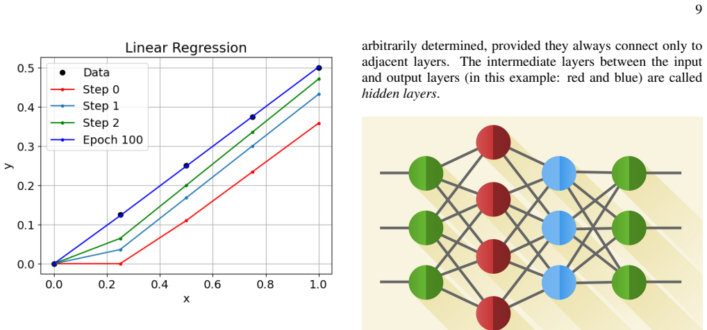
- [Section II.A.2, linear regression walkthrough] The step-by-step regression example is numerically inconsistent. Equation (11) initializes b = -0.138, but the batch computation uses b = -0.13; the first entry of wt+b is written as -0.138, which agrees with the former, not the latter, and for t = 0.25 the two choices give -0.01375 and -0.00575, respectively. After the first update the text reports w_new = 0.4906 and b_new = -0.1464, but using those updated weights the ReLU outputs are not the stated [0, 0.036, 0.178, 0.32, 0.46]; they are [0, 0, 0.0989, 0.2216, 0.3442], and the reported post-update loss 0.0643 does not follow from either set of numbers. Since the paper explicitly promises a step-by-step guide, these arithmetic errors need to be corrected and the whole walkthrough rechecked.
minor comments (7)
- [Abstract and Introduction] Grammar and spelling need a pass; examples include 'neural network and their basic concepts', 'Austrália' in the affiliation, and inconsistent capitalization in the enumerated list of applications.
- [Section II.A.1, Listing 1] The code uses variables x and y that are not defined in the snippet (the text defines x_j and y_j); as printed the code will raise a NameError. Listing 2 defines these variables correctly; the two listings should be made consistent.
- [Appendix A, near Table I] The sentence 'On Table I there are some of the main cost functions used in ML' refers to Table I, which actually lists activation functions; Table II is the cost-function table.
- [Section III.D] 'Lorentz attractors' should be 'Lorenz attractors'.
- [Figure 6 caption] The caption lists predictions at epochs 0, 1, 2, and 100 but refers only to red, green, and blue lines; please specify the color-to-epoch correspondence.
- [Section III.C and the abstract] The experiment estimates the dimensionality of the image manifold for a single simulated trajectory, but the text repeatedly says it estimates 'the dimensionality of the parameter space.' Please adjust the wording to avoid suggesting that the autoencoder is measuring the number of physical parameters of the pendulum.
- [Supplementary material entry [73]] The repository is cited without a commit hash or DOI; for a tutorial whose numerical claims readers are expected to reproduce, please pin the exact version.
Circularity Check
No circularity found: the four pendulum examples are externally validated against analytic solutions or the fitted equation itself, and no result reduces by construction to its inputs.
full rationale
The paper is a tutorial whose central demonstrations are known-answer tests rather than derivations from first principles. Example 1 fits g through the known small-angle solution (Eq. 25) and compares the fitted curve to the data; this is parameter estimation, not a circular prediction. Example 2 solves the harmonic-oscillator ODE with a PINN by minimizing the ODE residual (Eq. 28) plus initial and boundary terms, then checks against the analytic solution (Eq. 25); the validation target is external to the training loss. Example 3 trains an autoencoder on images generated from the pendulum ODE and checks that a one-dimensional latent space reconstructs them; the expected dimensionality is known in advance, so the exercise is a controlled demonstration rather than a self-referential derivation. Example 4 uses the standard SINDy-autoencoder loss (Eqs. 39-44) on data generated from Eq. (23), with a library that contains sin(z) and z; the recovered sparse equation is compared with the known pendulum equation. That is a benchmark of the method, not a prediction equivalent to its fitted inputs. The SINDy paragraph is internally inconsistent ('8 recovered the correct model' while also reporting recovered linear and mixed sin/z models), which is a reproducibility/correctness problem but not circularity. Section II's 'Universal Approximation (Kolmogorov-Arnold)' theorem (Eq. 15) is misstated as written, conflating exact Kolmogorov-Arnold representation with approximate MLP universality; again this is a mathematical correctness issue, not circular reasoning. No load-bearing self-citations appear: the only author self-citation ([69]) is for an adapted figure, and the SINDy architecture and pendulum example are attributed to external works [17,106]. The notebooks [73] are offered as reproducibility support, not as the justification of any derived claim. Because no claim in the paper reduces by construction to its own inputs, the circularity score is 0.
Assumptions & free parameters
free parameters (7)
- Learning rate eta (perceptron example) =
0.01
- Learning rate eta (linear regression example) =
0.05
- Loss weights lambda_1, lambda_2, lambda_3 (SINDy) =
lambda_1=5e-4, lambda_2=5e-5, lambda_3=1e-5
- Sparsity threshold =
0.1
- Latent space dimensions (autoencoder) =
1 and 2
- Gravity g' (Example 1) =
Not reported
- SINDy coefficients Xi =
Recovered equation (23) in 8/10 runs
assumptions (6)
- standard math The chain rule and calculus of differentiable functions apply to network training (backpropagation).
- ad hoc to paper A two-layer neural network with enough neurons can approximate any continuous function (Theorem II.1).
- domain assumption The simple pendulum ODE d^2 theta/dt^2 + (g/l) sin theta = 0 describes the physical system.
- domain assumption For small angles, sin(theta) approximately equals theta.
- domain assumption The pendulum state can be described by a single variable theta(t), so one latent dimension should suffice for the autoencoder.
- domain assumption Images of the pendulum are generated from theta(t) and derivatives can be computed numerically from smooth images.
Cite this review
Pith. "Pith review of An introduction to Neural Networks for Physicists." pith.science (2026). https://pith.science/paper/7CM4CX3W
@misc{pith2026250513042,
  author       = {Pith},
  title        = {Pith review of: An introduction to Neural Networks for Physicists},
  year         = {2026},
  howpublished = {\url{https://pith.science/paper/7CM4CX3W}},
  note         = {Machine review of arXiv:2505.13042}
}
read the original abstract
Machine learning techniques have emerged as powerful tools to tackle various challenges. The integration of machine learning methods with Physics has led to innovative approaches in understanding, controlling, and simulating physical phenomena. This article aims to provide a practical introduction to neural network and their basic concepts. It presents some perspectives on recent advances at the intersection of machine learning models with physical systems. We introduce practical material to guide the reader in taking their first steps in applying neural network to Physics problems. As an illustrative example, we provide four applications of increasing complexity for the problem of a simple pendulum, namely: parameter fitting of the pendulum's ODE for the small-angle approximation; Application of Physics-Inspired Neural Networks (PINNs) to find solutions of the pendulum's ODE in the small-angle regime; Autoencoders applied to an image dataset of the pendulum's oscillations for estimating the dimensionality of the parameter space in this physical system; and the use of Sparse Identification of Non-Linear Dynamics (SINDy) architectures for model discovery and analytical expressions for the nonlinear pendulum problem (large angles).
Figures


Figures from the paper (15 more)




Reference graph
Works this paper leans on
-
[1]
i.e., each elementMij is the average of the elements of a2×2 submatrix ofB 4×4
Given a block of pixels from a larger image,B 4×4, i.e., a submatrix of the input data matrix, then 12 pooling(B4×4) =M 2×2, whereMij = 1 4 i+2,j+2X k=i,l=j Bkl. i.e., each elementMij is the average of the elements of a2×2 submatrix ofB 4×4
-
[2]
Note that after such an operation, the size of the processed input data is now com- pressed into a smaller matrix
From the same block of pixelsB 4×4, taking the largest of the elements of a2x2submatrixM ij = maxi+2,j+2 k=i,l=j (Bkl), provides a different kind of pooling. Note that after such an operation, the size of the processed input data is now com- pressed into a smaller matrix. Reducing the dimensionality of the data decreases the network’s processing time and ...
-
[3]
∆l′ = (y[n] l′ −ˆyl′) d dz[n] l′ fl′(z[n] l′ )(19)
Start by calculating the deviation of thelossfunction from the true value with respect to an outputland its derivative but applying the chain rule only once. ∆l′ = (y[n] l′ −ˆyl′) d dz[n] l′ fl′(z[n] l′ )(19)
-
[4]
(18) ∆l′←∆ l′ ˆM d dw[k] il z[k] l (20) 13
Now, since the derivatives d dz[k] l′ fl′(z[k] l′ )were calcu- lated during thefeedforwardstep where we computed fl′(z[k] l′ ), retrieve them from memory and update delta with the matrix composition ˆMfrom the equation. (18) ∆l′←∆ l′ ˆM d dw[k] il z[k] l (20) 13
-
[5]
03- Example 1,
Repeat steps 1 and 2 for alll ′. Now take the average of the resulting deltas∆, and update the weightw [k] il as we did in the equation.(5) e (6) w[k] il,new←w [k] il,old−η∆(21) b[k] l,new←b [k] l,old−η∆(22) Thebackpropagationalgorithm has limitations that can compromise its performance and applicability in deep NNs. One of the main limitations is the pro...
-
[6]
Géron, A. (2017). Hands-on Machine Learning with Scikit- Learn, Keras, and TensorFlow. O’Reilly Media. ISBN: 978-1- 4920-3264-9
2017
-
[7]
Brunton, S. L. and Kutz, J. N. Data Driven Science and Engi- neering. (2017)
2017
-
[8]
Reviews of Modern Physics.91, 045002 (2019)
Carleo, Giuseppe et al, Machine learning and the physical sci- ences. Reviews of Modern Physics.91, 045002 (2019)
2019
Show all 108 references
-
[9]
Schmidhuber, J. (2015). Deep learning in neural networks: An overview. Neural Networks, 61, 85-117. ISSN 0893-6080
2015
-
[10]
Uddin, S., Haque, I., Lu, H. et al. Comparative performance analysis of K-nearest neighbour (KNN) algorithm and its dif- ferent variants for disease prediction. Sci Rep 12, 6256 (2022)
2022
-
[11]
k-Nearest neighbour classifiers: (with Python examples)
Cunningham, Padraig, and Sarah Jane Delany. "k-Nearest neighbour classifiers: (with Python examples)." arXiv preprint arXiv:2004.04523 (2020)
2020 arXiv
-
[12]
An Introduction to Logistic Regression Analysis and Reporting
Peng, Chao-Ying Joanne, et al. “An Introduction to Logistic Regression Analysis and Reporting.” The Journal of Educa- tional Research, vol. 96, no. 1, pp. 3–14,(2002)
2002
-
[13]
Logistic Regression: From Art to Sci- ence
Bertsimas, D., King, A. Logistic Regression: From Art to Sci- ence. Statistical Science, 32, 367-384, (2017)
2017
-
[14]
What is a support vector machine?
Noble, W. What is a support vector machine?. Nat Biotechnol 24, 1565–1567 (2006)
2006
-
[15]
C., de Carvalho, A
Lorena, A. C., de Carvalho, A. C. P. L. F. Uma Introdução às Support Vector Machines. Revista De Informática Teórica E Aplicada, 14(2), 43–67,(2007)
2007
-
[16]
Decision trees: a recent overview
Kotsiantis, S.B. Decision trees: a recent overview. Artif Intell Rev 39, 261–283 (2013)
2013
-
[17]
What are decision trees? Nat Biotechnol
Kingsford C, Salzberg SL. What are decision trees? Nat Biotechnol. Sep;26(9):1011-3 (2008)
2008
-
[18]
Introduction to machine learning for the sciences
Neupert, Titus, et al. "Introduction to machine learning for the sciences." arXiv preprint arXiv:2102.04883 (2021)
2021 arXiv
-
[19]
Machine Learning Algorithms: A ref- erence guide to popular algorithms for data science and ma- chine learning
Giuseppe Bonaccorso. Machine Learning Algorithms: A ref- erence guide to popular algorithms for data science and ma- chine learning. Packt Publishing, (2017)
2017
-
[20]
Machine learning and quantum devices
Marquardt, F. Machine learning and quantum devices. SciPost Physics Lecture Notes (2021)
2021
-
[21]
and Courville, A
Goodfellow, I., Bengio, Y . and Courville, A. Deep Learning. MIT Press (2016). Available at: http://www.deeplearningbook.org
2016
-
[22]
Champion, K., Lusch, B., Kutz, J. N. and Brunton, S. L. 22 Data-driven discovery of coordinates and governing equa- tions. Proc. Natl. Acad. Sci. U.S.A. 116, 22445–22451 (2019)
2019
-
[23]
Silver, D., Huang, A., Maddison, C. et al. Mastering the game of Go with deep neural networks and tree search. Nature 529, 484–489 (2016). https://doi.org/10.1038/nature16961
2016 doi
-
[24]
Mnih, V ., Kavukcuoglu, K., Silver, D. et al. Human-level control through deep reinforcement learning. Nature 518, 529–533 (2015). https://doi.org/10.1038/nature14236
2015 doi
- [25]
-
[26]
Gligorov, V V and Williams, M, Efficient, reliable and fast high-level triggering using a bonsai boosted decision tree, Journal of Instrumentation.02, vol 8
-
[27]
and Whiteson, D
Baldi, P., Sadowski, P. and Whiteson, D. Searching for exotic particles in high-energy physics with deep learning. Nat Com- mun 5, 4308 (2014)
2014
-
[28]
A living re- view of machine learning for particle physics
Feickert, Matthew, and Benjamin Nachman. "A living re- view of machine learning for particle physics." arXiv preprint arXiv:2102.02770 (2021)
2021 arXiv
-
[29]
Machine learning phases of matter
Carrasquilla, J., Melko, R. Machine learning phases of matter. Nature Phys 13, 431–434 (2017)
2017
-
[30]
and Huber, S
Van Nieuwenburg, E., Liu, YH. and Huber, S. Learning phase transitions by confusion. Nature Phys 13, 435–439 (2017)
2017
-
[31]
S., Isayev, O., Roitberg, A
Smith, J. S., Isayev, O., Roitberg, A. E. (2017). ANI-1: an ex- tensible neural network potential with DFT accuracy at force field computational cost. Chemical Science, 8(4), 3192-3203. The Royal Society of Chemistry
2017
-
[32]
Physics-informed machine learning: A survey on problems, methods and applications
Hao, Zhongkai, et al. "Physics-informed machine learning: A survey on problems, methods and applications." arXiv preprint arXiv:2211.08064 (2022)
2022 arXiv
-
[33]
Physics-Informed machine learning,
G. E. Karniadakis, I. G. Kevrekidis, L. Lu, P. Perdikaris, S. Wang, and L. Yang, “Physics-Informed machine learning,” Nature Reviews Physics, vol. 3, no. 6, pp. 422–440, 2021
2021
-
[34]
When physics meets machine learn- ing: A survey of physics-informed machine learning
Meng, Chuizheng, et al. "When physics meets machine learn- ing: A survey of physics-informed machine learning." arXiv preprint arXiv:2203.16797 (2022)
2022 arXiv
-
[35]
Scientific machine learning through physics–informed neural networks: Where we are and what’s next
Cuomo, Salvatore, et al. "Scientific machine learning through physics–informed neural networks: Where we are and what’s next." Journal of Scientific Computing 92.3 (2022): 88
2022
-
[36]
Physics-guided, physics-informed, and physics-encoded neural networks in scientific comput- ing
Faroughi, Salah A., et al. "Physics-guided, physics-informed, and physics-encoded neural networks in scientific comput- ing." arXiv preprint arXiv:2211.07377 (2022)
2022 arXiv
-
[37]
Physics informed neural networks (pinns) for fluid mechan- ics: A review,
S. Cai, Z. Mao, Z. Wang, M. Yin, and G. E. Karniadakis, “Physics informed neural networks (pinns) for fluid mechan- ics: A review,” arXiv preprint arXiv:2105.09506, 2021
2021 arXiv
-
[38]
A Review of Physics-Informed Machine Learning in Fluid Mechanics
Sharma, P.; Chung, W.T.; Akoush, B.; Ihme, M. A Review of Physics-Informed Machine Learning in Fluid Mechanics. Energies 2023, 16, 2343
2023
-
[39]
Uncertainty quantification in scientific machine learning: Methods, metrics, and comparisons,
A. F. Psaros, X. Meng, Z. Zou, L. Guo, and G. E. Kar- niadakis, “Uncertainty quantification in scientific machine learning: Methods, metrics, and comparisons,” arXiv preprint arXiv:2201.07766, 2022
2022 arXiv
-
[40]
Physics-guided deep learning for dynam- ical systems: A survey,
R.WangandR.Yu,“Physics-guided deep learning for dynam- ical systems: A survey,” arXiv preprint arXiv:2107.01272, 2021
2021 arXiv
-
[41]
Neural networks in quantum many-body physics: a hands-on tutorial
Carrasquilla, Juan, and Giacomo Torlai. "Neural networks in quantum many-body physics: a hands-on tutorial." arXiv preprint arXiv:2101.11099 (2021)
2021 arXiv
-
[42]
Artificial neural networks for photonic applications—from algorithms to implementation: tutorial,
Pedro Freire, Egor Manuylovich, Jaroslaw E. Prilepsky, and Sergei K. Turitsyn, "Artificial neural networks for photonic applications—from algorithms to implementation: tutorial," Adv. Opt. Photon. 15, 739-834 (2023)
2023
-
[43]
Froim, S.; Yosef, Erez ; Giryes, Raja ;Bahabad, Alon
Hadad, B. ; Froim, S.; Yosef, Erez ; Giryes, Raja ;Bahabad, Alon. Deep learning in optics - a tutorial. Journal of Optics
-
[44]
A Review of Optical Neural Networks
Zhang, D.; Tan, Z. A Review of Optical Neural Networks. Appl. Sci. 2022, 12, 5338
2022
-
[45]
Quantum Computing and Ma- chine Learning on an Integrated Photonics Platform
Zhu, H.; Lin, H.; Wu, S.; Luo, W.; Zhang, H.; Zhan, Y .; Wang, X.; Liu, A.; Kwek, L.C. Quantum Computing and Ma- chine Learning on an Integrated Photonics Platform. Informa- tion 2024, 15, 95
2024
-
[46]
Palmieri, A.M., Kovlakov, E., Bianchi, F. et al. Experimental neural network enhanced quantum tomography. npj Quantum Inf 6, 20 (2020)
2020
-
[47]
Adaptive quantum state tomogra- phy with neural networks
Quek, Y ., Fort, S.; Ng, H.K. Adaptive quantum state tomogra- phy with neural networks. npj Quantum Inf 7, 105 (2021)
2021
-
[49]
Three ways to solve par- tial differential equations with neural networks—a review,
J. Blechschmidt and O. G. Ernst, “Three ways to solve par- tial differential equations with neural networks—a review,” GAMM-Mitteilungen, vol. 44, no. 2, p. e202100006,( 2021)
2021
-
[50]
In- tegrating physics-based modeling with machine learning: A survey,
J. Willard, X. Jia, S. Xu, M. Steinbach, and V . Kumar, “In- tegrating physics-based modeling with machine learning: A survey,” arXiv preprint arXiv:2003.04919, vol. 1, no. 1, pp. 1–34, 2020
2003 arXiv
-
[51]
Adv.6,eaay2631(2020)
Silviu-Marian Udrescu, Max Tegmark ,AI Feynman: A physics-inspired method for symbolic regression.Sci. Adv.6,eaay2631(2020)
2020
-
[53]
Li, Z., Kovachki, N.B., Azizzadenesheli, K., Liu, B., Bhat- tacharya, K., Stuart, A.M., and Anandkumar, A. (2020). Fourier Neural Operator for Parametric Partial Differential Equations. ArXiv, abs/2010.08895
2020 arXiv
-
[54]
Optical machine learning with inco- herent light and a single-pixel detector
Jiao, Shuming, et al. "Optical machine learning with inco- herent light and a single-pixel detector." Optics letters 44.21 (2019): 5186-5189
2019
-
[55]
Arti- ficial intelligence and machine learning in optics: tutorial,
Ksenia Yadav, Serge Bidnyk, and Ashok Balakrishnan, "Arti- ficial intelligence and machine learning in optics: tutorial," J. Opt. Soc. Am. B 41, 1739-1753 (2024)
2024
-
[56]
Neuralpde: Automating physics- informed neural networks (pinns) with error approximations
Zubov, Kirill, et al. "Neuralpde: Automating physics- informed neural networks (pinns) with error approximations." arXiv preprint arXiv:2107.09443 (2021)
2021 arXiv
-
[57]
Adv.6,eaay2631(2020).DOI:10.1126/sciadv.aay2631
Silviu-Marian Udrescu, Max Tegmark, AI Feynman: A physics-inspired method for symbolic regression.Sci. Adv.6,eaay2631(2020).DOI:10.1126/sciadv.aay2631
2020 doi
-
[58]
PhyCV: the first physics-inspired com- puter vision library
Zhou, Yiming, et al. "PhyCV: the first physics-inspired com- puter vision library." arXiv preprint arXiv:2301.12531 (2023)
2023 arXiv
-
[59]
Physics-informed computer vision: A review and perspectives
Banerjee, Chayan, et al. "Physics-informed computer vision: A review and perspectives." ACM Computing Surveys (2024)
2024
-
[60]
ChatGPT: A comprehensive review on background, applications, key challenges, bias, ethics, limita- tions and future scope
Ray, Partha Pratim. “ChatGPT: A comprehensive review on background, applications, key challenges, bias, ethics, limita- tions and future scope.” Internet of Things and Cyber-Physical Systems (2023)
2023
-
[61]
Convolutional neu- ral networks for image classification,
N. Jmour, S. Zayen and A. Abdelkrim, "Convolutional neu- ral networks for image classification," 2018 International Con- ference on Advanced Systems and Electric Technologies (IC ASET), Hammamet, Tunisia, pp. 397-402,(2018)
2018
-
[62]
The Application and Im- provement of Deep Neural Networks in Environmental Sound Recognition
Lin, Y .-K.; Su, M.-C.; Hsieh, Y .-Z. The Application and Im- provement of Deep Neural Networks in Environmental Sound Recognition. Appl. Sci., 10, 5965, (2020)
2020
-
[63]
Natural Language Processing with Improved Deep Learning Neural Networks
YiTao Zhou, "Natural Language Processing with Improved Deep Learning Neural Networks", Scientific Programming, 8 23 pages, (2022)
2022
-
[64]
Fisher,R. A.. (1988). Iris. UCI Machine Learning Repository. https://doi.org/10.24432/C56C76
1988 doi
-
[65]
Scikit-learn: Machine learning in Python
Pedregosa, Fabian, et al. "Scikit-learn: Machine learning in Python." the Journal of machine Learning research 12: 2825- 2830, (2011)
2011
-
[66]
Understanding the dif- ficulty of training deep feedforward neural networks
Glorot, Xavier, and Yoshua Bengio. "Understanding the dif- ficulty of training deep feedforward neural networks." Pro- ceedings of the thirteenth international conference on artificial intelligence and statistics. JMLR Workshop and Conference Proceedings, (2010)
2010
-
[67]
Review and comparison of commonly used activation functions for deep neural networks
Szandała, Tomasz. "Review and comparison of commonly used activation functions for deep neural networks." Bio- inspired neurocomputing: 203-224, (2021)
2021
-
[68]
Implicit neural representations with periodic activation functions
Sitzmann, Vincent, et al. "Implicit neural representations with periodic activation functions." Advances in neural information processing systems 33: 7462-7473. (2020)
2020
-
[69]
Dawid, A. et al. Modern applications of machine learning in quantum sciences. arXiv:2204.04198 (2022)
2022
-
[70]
A review on applications of genetic algorithm for artificial neural network
Al Tobi, Maamer Ali Saud, et al. "A review on applications of genetic algorithm for artificial neural network." International Journal of Advance Computational Engineering and Network- ing 4.9 (2016): 50-54
2016
-
[71]
Neural network structure optimization by simulated annealing
Kuo, Chun Lin, Ercan Engin Kuruoglu, and Wai Kin Victor Chan. "Neural network structure optimization by simulated annealing." Entropy 24.3 (2022): 348
2022
-
[72]
An Overview of Stochastic Gradient De- scent in Machine Learning
del Rosario, Mason. "An Overview of Stochastic Gradient De- scent in Machine Learning." (2019)
2019
-
[73]
Survey of optimization algorithms in modern neural net- works
Abdulkadirov, Ruslan, Pavel Lyakhov, and Nikolay Nagornov. "Survey of optimization algorithms in modern neural net- works." Mathematics 11.11 (2023): 2466
2023
-
[74]
Pulse modulation for enhanced control in NMR-based Quantum Devices
Café de Miranda, G. Pulse modulation for enhanced control in NMR-based Quantum Devices. Universidade Federal do ABC, Janeiro 2024
2024
-
[75]
Grid search, random search, genetic algorithm: a big comparison for NAS
Liashchynskyi, Petro, and Pavlo Liashchynskyi. "Grid search, random search, genetic algorithm: a big comparison for NAS." arXiv preprint arXiv:1912.06059 (2019)
2019 arXiv
-
[76]
An overview of stochastic gradient-based methods
Gower, Robert, and Telecom Paris. "An overview of stochastic gradient-based methods." (2019)
2019
-
[77]
Kingma and Jimmy Ba
Diederik P. Kingma and Jimmy Ba. Adam: A Method for Stochastic Optimization. arXiv:1412.6980, 2014
2014 arXiv
-
[78]
Café de Miranda, G., Lima, G. G. Notebooks acompan- hando o artigo. Repositório GitHub,https://github. com/Coffee4MePlz/Notebooks_NN_Physics
-
[79]
Introduction to Neural Network
Safrin. Introduction to Neural Network. Medium, https://medium.com/@safrin1128/ introduction-to-neural-network-9fdff448f43f. Acessado em: 15 de fevereiro de 2025
2025
-
[80]
Learning internal representations by error propagation,
D. E. Rumelhart, G. E. Hinton, and R. J. Williams, “Learning internal representations by error propagation,” California Uni- vSan Diego La Jolla Inst for Cognitive Science, Tech. Rep., (1985)
1985
-
[81]
Hinton, G
LeCun, Y ., Bengio, Y . Hinton, G. Deep learning. Nature 521, 436–444 (2015)
2015
-
[82]
Long short-term memory,
S. Hochreiter and J. Schmidhuber, “Long short-term memory,” Neural computation, vol. 9, no. 8, pp. 1735–1780, (1997)
1997
-
[83]
A survey of transformers
Lin, Tianyang, et al. "A survey of transformers." AI open 3: 111-132 (2022)
2022
-
[84]
An introduction to autoencoders
Michelucci, Umberto. "An introduction to autoencoders." arXiv preprint arXiv:2201.03898 (2022)
2022 arXiv
-
[85]
Electronics 8(3), (2019)
Alom MZ, Taha TM, Yakopcic C, et al, A state-of-the-art survey on deep learning theory and architectures. Electronics 8(3), (2019)
2019
-
[86]
Neural Network Architectures
Herberg, Evelyn. "Neural Network Architectures." arXiv preprint arXiv:2304.05133 (2023)
2023 arXiv
-
[87]
Hopfield networks is all you need
Ramsauer, Hubert, et al. "Hopfield networks is all you need." arXiv preprint arXiv:2008.02217 (2020)
2020 arXiv
-
[88]
Liu, Z. et al. KAN: Kolmogorov-Arnold Networks. Preprint at http://arxiv.org/abs/2404.19756 (2024)
2024 arXiv
-
[89]
Pytorch: An imperative style, high- performance deep learning library
Paszke, Adam, et al. "Pytorch: An imperative style, high- performance deep learning library." Advances in neural infor- mation processing systems 32 (2019)
2019
-
[90]
Tensor- Flow: Large-scale machine learning on heterogeneous sys- tems, Software available from tensorflow.org
Martín Abadi, Ashish Agarwal, Paul Barham, et al. Tensor- Flow: Large-scale machine learning on heterogeneous sys- tems, Software available from tensorflow.org. (2015)
2015
-
[91]
JAX: composable transformations of Python+ NumPy programs
Bradbury, James, et al. "JAX: composable transformations of Python+ NumPy programs." (2018)
2018
-
[92]
Automatic differentiation in ma- chine learning: a survey
Baydin, Atilim Gunes, et al. "Automatic differentiation in ma- chine learning: a survey." Journal of machine learning re- search 18.153 (2018): 1-43
2018
-
[93]
Artigos no Medium
Pham, K. Artigos no Medium. Medium,https:// medium.com/@khang.pham.exxact. Acessado em: 15 de fevereiro de 2025
2025
-
[94]
Im- ageNet Classification with Deep Convolutional Neural Net- works
Alex Krizhevsky, Ilya Sutskever, Geoffrey E Hinton. "Im- ageNet Classification with Deep Convolutional Neural Net- works". In:Advances in Neural Information Processing Sys- tems, vol. 25, ed. by F. Pereira et al., Curran Associates, Inc., 2012
2012
-
[95]
VisualBackProp: efficient visualization of CNNs
Mariusz Bojarski, Anna Choromanska, Krzysztof Choroman- ski, Bernhard Firner, Larry Jackel, Urs Muller, Karol Zieba. "VisualBackProp: efficient visualization of CNNs". (2017). arXiv preprint arXiv:1611.05418
2017 arXiv
-
[96]
Feature Detection with Automatic Scale Selec- tion
Lindeberg, T. Feature Detection with Automatic Scale Selec- tion. Int. J. Comput. Vis. 30, 79–116 (1998)
1998
-
[97]
and Murphey, Y .L
Park, J.M. and Murphey, Y .L. (2008). Edge Detection in Grayscale, Color, and Range Images. In Wiley Encyclopedia of Computer Science and Engineering, B.W. Wah (Ed.)
2008
-
[98]
Detecting salient blob-like image structures and their scales with a scale-space primal sketch: A method for focus-of-attention
Lindeberg, T. Detecting salient blob-like image structures and their scales with a scale-space primal sketch: A method for focus-of-attention. Int. J. Comput. Vis. 11, 283–318 (1993)
1993
-
[99]
Neocognitron: A self-organizing neural net- work model for a mechanism of pattern recognition unaffected by shift in position
Fukushima, K. Neocognitron: A self-organizing neural net- work model for a mechanism of pattern recognition unaffected by shift in position. Biol. Cybernetics 36, 193–202 (1980)
1980
-
[100]
Basodi, C
S. Basodi, C. Ji, H. Zhang and Y . Pan. Gradient amplification: An efficient way to train deep neural networks. Big Data Min- ing and Analytics, vol. 3, no. 3, pp. 196-207, Sept. 2020, doi: 10.26599/BDMA.2020.9020004
2020
-
[101]
Bashir, D., Montañez, G.D., Sehra, S., Segura, P.S., Lauw, J. (2020). An Information-Theoretic Perspective on Overfitting and Underfitting. In: Gallagher, M., Moustafa, N., Lakshika, E. (eds) AI 2020: Advances in Artificial Intelligence. AI 2020. Lecture Notes in Computer Scie...
2020
-
[102]
Addressing the loss-metric mismatch with adaptive loss alignment
Huang, Chen, et al. "Addressing the loss-metric mismatch with adaptive loss alignment." International conference on ma- chine learning. PMLR, 2019
2019
-
[103]
Plateau phenomenon in gradient descent training of RELU networks: Explanation, quantification, and avoidance
Ainsworth, Mark, and Yeonjong Shin. "Plateau phenomenon in gradient descent training of RELU networks: Explanation, quantification, and avoidance." SIAM Journal on Scientific Computing 43.5 (2021): A3438-A3468
2021
-
[104]
Which neural net architectures give rise to ex- ploding and vanishing gradients?
Hanin, Boris. "Which neural net architectures give rise to ex- ploding and vanishing gradients?." Advances in neural infor- mation processing systems 31 (2018)
2018
-
[105]
Lusch, B., Kutz, J. N. and Brunton, S. L. Deep learning for universal linear embeddings of nonlinear dynamics. Nat Com- mun 9, 4950 (2018)
2018
-
[106]
Gamelin, T. W. Complex Analysis. Springer New York, New York, NY (2001). doi:10.1007/978-0-387-21607-2. 24
2001 doi
-
[108]
and Manzagol, P.-A
Vincent, P., Larochelle, H., Bengio, Y . and Manzagol, P.-A. Extracting and composing robust features with denoising au- toencoders. in Proceedings of the 25th international confer- ence on Machine learning - ICML ’08 1096–1103 ACM Press (2008). doi:10.1145/1390156.1390294
2008
-
[109]
C Gheller, F Vazza, Convolutional deep denoising au- toencoders for radio astronomical images, Monthly Notices of the Royal Astronomical Society, V ol- ume 509, Issue 1, January 2022, Pages 990–1009, https://doi.org/10.1093/mnras/stab3044
2022 doi
-
[110]
and Petruccione, F
Schuld, M. and Petruccione, F. Machine Learning with Quan- tum Computers (2021)
2021
-
[111]
SINDy Pendulum
Sillano, Pietro. SINDy Pendulum. Github repositoryhttps: //github.com/pietro-sillano/SindyPendulum APPENDIX A - CALCULA TION OF THE COST FUNCTION Activation Function f(x) Derivative Sigmoid 1 1+e−x f′(x) =f(x)(1−f(x)) Tanh tanh(x) f′(x) = 1−f(x) 2 ReLU max(0,x) f′(x) = ( 1ifx>...
Reviewed August 15, 2026 · model on record in the stance chip above.
Discussion (0). Continue with ORCID to comment.