REVIEW 3 major objections 4 minor 29 references
Scalable Bayesian Monte Carlo: fast uncertainty estimation beyond deep ensembles
T0 review · 3 major / 4 minor · reviewed 2026-08-15 · deepseek-v4-flash
Pith's one-line read At the same wall-clock cost as a deep ensemble, SBMC matches its accuracy and supplies epistemic uncertainty that deep ensembles miss.
desk verdict Solid empirical contribution with a misleading wall-clock claim: SBMC's cost is roughly double deep ensembles, but the UQ gains on IMDb are real. read the letter →
The pith
A machine-rendered reading of the paper's core claim, the machinery that carries it, and where it could break.
The reading
What carries the argument
The load-bearing object is the anchored posterior $\pi_s(\theta) \propto L(\theta)\,\mathcal{N}(\theta;\theta_{\mathrm{MAP}}, s v I_d)$, with scalar interpolation parameter $s\in[0,1]$ (the paper uses $\alpha(s)=\mathbf{1}_{s<1/2}$ and $\Sigma(s)=s v I_d$ in the isotropic case). It turns an intractable posterior into a family of targets interpolating between a point mass at the MAP and the full posterior; small $s$ flattens the likelihood relative to the anchored prior, improves Hessian conditioning, and lets short parallel chains mix. The companion machinery is the parallel BMC layer: $P$ independent executions of SMC$_{\parallel}$ or MCMC$_{\parallel}$, each with $N$ particles or chains, combined through a weighted ratio estimator without inter-process communication.
What would settle it
On a small problem where a long gold-standard HMC run is feasible, compute the rank correlation between SBMC's per-input epistemic entropy at the recommended default $s=0.1$ and the gold-standard posterior's over correct, incorrect, and OOD inputs; a weak or negative correlation on the incorrect/OOD subset would falsify the claim that the anchored posterior recovers useful epistemic uncertainty.
Extended reading notes
Core claim
The paper's central claim is that, for a fixed time budget measured in epochs, targeting the MAP-anchored posterior $\pi_s(\theta) \propto L(\theta)\mathcal{N}(\theta;\theta_{\mathrm{MAP}}, s v I_d)$ with parallel SMC or MCMC recovers essentially the accuracy of the point estimator while supplying an epistemic-uncertainty signal that deep ensembles systematically underestimate. In the reported numbers, SBMC at roughly 160 to 200 epochs reaches accuracy comparable to deep ensembles and, when its posterior features are fed to a confidence meta-classifier, achieves higher F1 and AUC-ROC for detecting misclassifications and out-of-distribution inputs; the long-run gold-standard HMC posterior remains the stated ceiling. The interpolation parameter $s$ is the control knob: $s=0$ collapses to the MAP, $s=1$ is the true posterior, and intermediate values trade a small bias for much faster mixing.
Load-bearing premise
The load-bearing premise is that a single scalar anchoring strength, chosen per dataset and justified only by a heuristic sketch, makes the approximate posterior's epistemic-entropy ranking of mistakes and out-of-distribution inputs trustworthy.
Editorial extensions
If this is right
- At equal per-chain epoch cost, SBMC matches deep-ensemble accuracy on MNIST7, IMDb, and CIFAR10 while delivering markedly higher epistemic entropy, especially on out-of-distribution inputs.
- Epistemic entropy from the SBMC posterior ranks individual predictions: incorrect and OOD examples receive higher scores, so the signal can drive abstention decisions via a confidence meta-classifier.
- Because the sampler is consistent for the anchored target, any Bayesian Monte Carlo algorithm, such as SMC$_{\parallel}$, HMC$_{\parallel}$, or future stochastic-gradient variants, can be dropped into SBMC without changing the estimator.
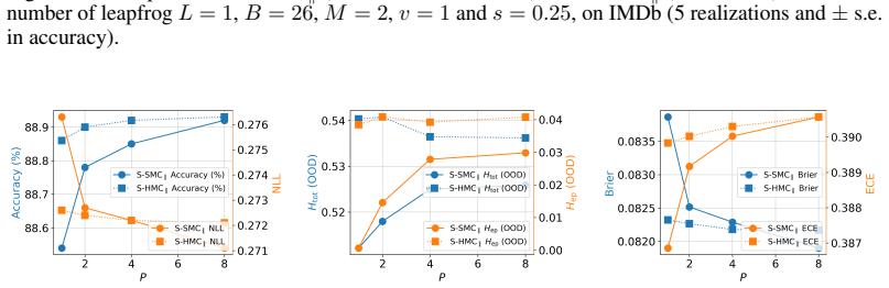
- Scaling the number of parallel processes $P$ improves uncertainty estimates, with S-SMC$_{\parallel}$ improving more sharply than S-HMC$_{\parallel}$ as $P$ grows.
Reading between the lines
- The paper's own experiments tune $s$ per dataset (0.05 to 0.35), so a fully automatic selection rule for $s$, for example empirical Bayes on the marginal likelihood or a cross-validated grid, is the natural next step; without it, the scalable claim carries an extra tuning cost.
- The anchored-posterior trick is a post-hoc add-on: once a MAP or deep ensemble exists, short chains on the last layer or on LoRA adapters could give the same UQ benefit to frozen pretrained models, which is the direction the GPT-2 appendix gestures at.
- A minimal deployment test would ask whether a single epistemic-entropy threshold, without the seven-feature meta-classifier, already separates OOD from in-domain inputs; if it does, SBMC's practical overhead drops further.
Signed reviews
Editorial analysis
A structured set of objections, weighed in public.
Referee Report
Summary. The paper introduces Scalable Bayesian Monte Carlo (SBMC), a method for Bayesian deep learning that combines a MAP-anchored Gaussian prior with an interpolation parameter s, and parallel SMC or MCMC samplers that target the resulting anchored posterior. The authors claim that, for the same wall-clock time as deep ensembles (DE), SBMC delivers comparable or better accuracy and substantially improved epistemic uncertainty quantification, demonstrated on MNIST7, IMDb, CIFAR-10, and a preliminary GPT-2 experiment. The paper includes extensive experiments with 5 realizations, ablations over s and P, and comparisons with MAP, DE, MC Dropout, Laplace approximation, and SWA, as well as long-run HMC as a gold standard.
Significance. If the headline claim were fully supported, SBMC would be a practically valuable contribution: it offers a sampling-based method with formal consistency for its target, while providing epistemic UQ at a cost comparable to a popular heuristic (DE). The empirical study is unusually thorough for this line of work: standard errors from 5 realizations are reported, many baselines are included, and the sensitivity to the tuning parameters s and P is examined. The authors are also transparent about the approximate nature of the target and explicitly flag the heuristic character of the theoretical sketch. However, the central 'same wall-clock time' claim is not supported by the paper's own cost accounting, which uses worker-epochs rather than wall-clock time. This is a load-bearing issue that must be resolved before the paper's main contribution can be accepted as stated.
major comments (3)
- [Section 2, Table 1, Abstract] The claim that SBMC matches deep ensembles 'for the same wall-clock time' is contradicted by the paper's own accounting. Section 2 defines time cost as 'simulation time per chain/particle' in epochs, a hardware-agnostic proxy, and the Total Cost column in Table 1 counts MAP epochs plus (sampling epochs × N × P). On identical parallel hardware, the wall-clock critical path for S-HMC∥ (P=1, N=10) is 160 epochs for the MAP phase plus 160 epochs for the parallel sampling phase, i.e. 320 epochs, versus 176 epochs for a deep ensemble whose members run in parallel. The text near Table 1 even concedes 'SBMC methods require the MAP estimator, so their total time cost is roughly double,' which directly contradicts the abstract's phrasing. The comparison should be re-framed as equal worker-epochs or total compute, and the abstract and title-level claims should be adjusted accordingly.
- [Table 1, HMC (GS) row] The NLL for the 200,000-epoch HMC gold standard is listed as 1.94±0.004, whereas Table 8 reports 1.942e-1 (0.1942) for the same setting. The decimal error in Table 1 makes the gold-standard look dramatically worse and is inconsistent with the supporting tables. This should be corrected, and the surrounding text should be checked for similar transcription errors.
- [Appendix C and Section 5] The theoretical justification is explicitly heuristic: Appendix C states 'let's suppose we wave our hands' in deriving the link to a Laplace approximation, and Section 5 recommends treating convergence heuristically because the target is not the posterior for s<1. The empirical UQ gain is thus an empirical observation for an approximate, data-dependent target, not a consequence of a formal theory. The paper should state this limitation more prominently in the abstract and introduction, so that readers do not infer a principled derivation of the reported UQ improvement.
minor comments (4)
- [Section 2, Eq. (2)] The symbol π0 is used both for the original prior N(0,V) and for the anchored prior N(α θ_MAP, Σ(s)), which causes confusion. Please use distinct notation, e.g. π_0^orig and π_0^anch.
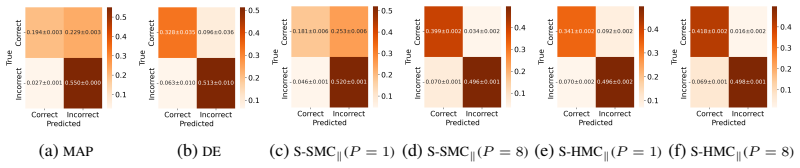
- [Figure 1 caption] The caption says 'every method runs for 25 epochs except the Gold-Standard,' which is inconsistent with Table 1 where MNIST7 runs are 160–178 epochs. Please clarify the dataset or setting to which the 25-epoch statement applies.
- [Tables with bolding] The phrase 'bold the first 30% data in mean' (e.g. in Tables 4–7) is unclear. Please explain what the bolding indicates and why the 30% cutoff is used.
- [References] Some references are incomplete, e.g. 'Qiu et al.' appears without a year or venue. Please normalize all citations.
Circularity Check
No circular derivation: the anchored posterior is a transparent approximation; the only flagged issue is a minor non-load-bearing self-citation, while the wall-clock claim is a correctness concern rather than circularity.
-
other
[Section 2, paragraph after Algorithm 1 (parallel speed-up motivation)]
"Parallel implementations of consistent BMC algorithms like SMC∥ and HMC∥ improve time cost with near linear speed-up [Liang et al., 2025], but each process still needs to run for a long time, as seen in Figure 1 (c)."
This is a self-citation by overlapping authors for the near-linear parallel speed-up claim used in the scalability motivation. It is flagged only as a minor self-citation, not as a load-bearing circular step: the paper's own ablations over P (Appendix H) independently show that increasing P improves accuracy and UQ at fixed per-chain cost, and the anchored-posterior construction does not reduce to the cited speed-up.
full rationale
The paper's central target is the anchored posterior in (3), π(θ) ∝ L(θ) N(θ; α(s)θ_MAP, s v I), with θ_MAP estimated from the same data. This makes the epistemic entropy a property of a data-dependent approximate target, not the true posterior, but the paper explicitly and repeatedly disclaims that it targets the posterior for s < 1: 'since the method no longer targets the posterior for any s < 1, we would recommend adopting a heuristic approach to convergence as with other SOTA methods, rather than chasing more rigorous convergence guarantees.' The sampler consistency for the anchored target is standard, and the UQ claims are benchmarked against gold-standard HMC and held-out OOD/meta-training labels, so no fitted parameter is renamed as a prediction. The one same-author citation, [Liang et al., 2025], supports near-linear parallel speed-up; it is not machine-checked here, but the paper's own P-ablation results provide independent empirical support, so it is not load-bearing for the central method. The abstract's 'same wall-clock time' statement is not supported by Table 1, which counts worker-epochs and adds a serial MAP phase, as the paper itself concedes that 'SBMC methods require the MAP estimator, so their total time cost is roughly double'; however, this is an accounting and correctness issue, not a circular reduction of a derivation to its inputs.
Assumptions & free parameters
free parameters (3)
- s (interpolation parameter) =
0.1 (MNIST7), 0.35 (IMDb with v=1), 0.05 (CIFAR10)
- v (prior variance) =
0.1 (MNIST7), 0.025 or 1 (IMDb), 0.2 (CIFAR10)
- P (number of parallel chains/particles) =
1 or 8 in experiments; N=10 particles
assumptions (3)
- standard math MCMC and SMC samplers are asymptotically unbiased for their target distribution; the parallel estimators in (4)-(5) converge to the target pi_s as N goes to infinity.
- domain assumption Short chains with the chosen hyperparameters (leapfrog L=1, adaptive mutation steps) mix fast enough to make the estimators reliable at the reported compute budget.
- domain assumption The MAP estimator theta_MAP, computed on the same training data, is a suitable center for the posterior, so an anchored prior around it yields useful epistemic uncertainty.
Cite this review
Pith. "Pith review of Scalable Bayesian Monte Carlo: fast uncertainty estimation beyond deep ensembles." pith.science (2026). https://pith.science/paper/5327WUS4
@misc{pith2026250513585,
  author       = {Pith},
  title        = {Pith review of: Scalable Bayesian Monte Carlo: fast uncertainty estimation beyond deep ensembles},
  year         = {2026},
  howpublished = {\url{https://pith.science/paper/5327WUS4}},
  note         = {Machine review of arXiv:2505.13585}
}
abstract
This work introduces a new method designed for Bayesian deep learning called scalable Bayesian Monte Carlo (SBMC). The method is comprised of a model and an algorithm. The model interpolates between a point estimator and the posterior. The algorithm is a parallel implementation of sequential Monte Carlo sampler (SMC$_\parallel$) or Markov chain Monte Carlo (MCMC$_\parallel$). We collectively refer to these consistent (asymptotically unbiased) algorithms as Bayesian Monte Carlo (BMC), and any such algorithm can be used in our SBMC method. The utility of the method is demonstrated on practical examples: MNIST, CIFAR, IMDb. A systematic numerical study reveals that for the same wall-clock time as state-of-the-art (SOTA) methods like deep ensembles (DE), SBMC achieves comparable or better accuracy and substantially improved uncertainty quantification (UQ)--in particular, epistemic UQ. This is demonstrated on the downstream task of estimating the confidence in predictions, which can be used for reliability assessment or abstention decisions.
Figures


Figures from the paper (27 more)






Reference graph
Works this paper leans on
-
[1]
• SW A. We train with SGD (momentum = 0.9 ) for a 25-epoch warm-up, then perform SW A weight averaging with 1 sample per epoch, at a fixedswa_lr = 0.0005. • MC Dropout. A fixed 30% dropout in the fully-connected layer;10samples are used. • Laplace. We fit a Laplace approximation with a Kronecker-factored approximation of the Hessian8Daxberger et al. [2021...
work page 2021
-
[2]
URLhttps://arxiv.org/abs/2502.13923. Johnathan M. Bardsley, Antti Solonen, Heikki Haario, and Marko Laine. Randomize–then–optimize: A method for sampling from posterior distributions in nonlinear inverse problems.SIAM Journal on Scientific Computing, 36(4):A1895–A1910,
-
[3]
Table 3: Comparison of methods on test accuracy, NLL, and various entropy metrics for next-token prediction with GPT2 on tiny Shakespeare. Methods Accuracy (%) NLL Htot correct Htot incorrect Hep correct Hep incorrect MAP 38.66 3.166 1.554 3.605 0 0 S-HMC 39.36 3.083 1.571 3.612 0.047 0.077 A.2 Overcoming other computational bottlenecks Our sampler relies...
work page 2017
-
[6]
Pierre Del Moral.Feynman-kac formulae
URLhttps://arxiv.org/abs/2501.12948. Pierre Del Moral.Feynman-kac formulae. Springer,
-
[9]
Introduces Bernoulli-thinning (random inclusion) unbiased-likelihood estimators inside SMC
doi: 10.1214/20-BA1220. Introduces Bernoulli-thinning (random inclusion) unbiased-likelihood estimators inside SMC. Fredrik K Gustafsson, Martin Danelljan, and Thomas B Schon. Evaluating scalable Bayesian deep learning methods for robust computer vision. InProceedings of the IEEE/CVF conference on computer vision and pattern recognition workshops, pages 318–319,
-
[10]
Bridging language and items for retrieval and recommendation.arXiv preprint arXiv:2403.03952,
Yupeng Hou, Jiacheng Li, Zhankui He, An Yan, Xiusi Chen, and Julian McAuley. Bridging language and items for retrieval and recommendation.arXiv preprint arXiv:2403.03952,
-
[12]
URL https://arxiv.org/abs/ 2503.03734. Yanping Huang et al. GPipe: Efficient training of giant neural networks using pipeline parallelism. InNeurIPS,
-
[13]
Averaging weights leads to wider optima and better generalization
11 Pavel Izmailov, Dmitrii Podoprikhin, Timur Garipov, Dmitry Vetrov, and Andrew Gordon Wilson. Averaging weights leads to wider optima and better generalization. In34th Conference on Uncertainty in Artificial Intelligence 2018, UAI 2018, pages 876–885. Association For Uncertainty in Artificial Intelligence (AUAI),
work page 2018
Show all 29 references
-
[14]
S-SMC∥ (P= 8 chain withN= 10 ), S-HMC∥ (NP chains), DE (N models) and MAP, with fixed number of leapfrog L= 1 ,B= 26 ,M= 2 , v= 1ands= 0.35(5realizations)
Figure 10: Comparison of average total and epistemic entropy over four out-of-domain classes and correct/incorrect predictions in-domain for IMDb. S-SMC∥ (P= 8 chain withN= 10 ), S-HMC∥ (NP chains), DE (N models) and MAP, with fixed number of leapfrog L= 1 ,B= 26 ,M= 2 , v= 1a...
-
[15]
Comparison of parallel SMC and MCMC for Bayesian deep learning.arXiv preprint arXiv:2402.06173,
Xinzhu Liang, Joseph M Lukens, Sanjaya Lohani, Brian T Kirby, Thomas A Searles, Xin Qiu, and Kody JH Law. Comparison of parallel SMC and MCMC for Bayesian deep learning.arXiv preprint arXiv:2402.06173,
-
[18]
URL https://openai.com/ index/gpt-oss-model-card/. Theodore Papamarkou, Maria Skoularidou, Konstantina Palla, Laurence Aitchison, Julyan Arbel, David Dunson, Maurizio Filippone, Vincent Fortuin, Philipp Hennig, Aliaksandr Hubin, et al. Po- sition paper: Bayesian deep learning ...
-
[21]
Optimised annealed Sequential Monte Carlo samplers.arXiv preprint arXiv:2408.12057,
13 Saifuddin Syed, Alexandre Bouchard-Côté, Kevin Chern, and Arnaud Doucet. Optimised annealed Sequential Monte Carlo samplers.arXiv preprint arXiv:2408.12057,
-
[23]
A Future Directions The most obvious next step is UQ for modern large language models (LLMs) [DeepSeek-AI, 2025], where robustness and hallucination detection are crucial pain points [Vashurin et al., 2024]. It has been recently shown that high-quality entropy metrics are valu...
2025
-
[25]
use EB for fitting prior and likelihood variance in the context of transfer learning for regression, and then they extended this idea for building estimators from an ensemble of pre-trained models You et al. [2022]. The latter could naturally be combined with other ensemble ap...
2022
-
[26]
tune away
prior, and now it is time to incorporate the rest of the data (1−a)ℓ . The Hessian of our Laplace approximation is a∇2ℓ(θ) + 1 2(v/a) Id. This could be carried through rigorously, but for the sake of the argument, let’s suppose we wave our hands and swap outNtrainId for∇2ℓ(θ) ...
2025
-
[28]
The NN model and parameter prior for IMDb10 are built as follows • NN is followed by (i) no hidden layer, (ii) ReLU activation, (iii) a final linear layer, and (iv) softmax output
In other words, frozen weights from all-mpnet-base-v2 until the 768 dimensional [CLS] output. The NN model and parameter prior for IMDb10 are built as follows • NN is followed by (i) no hidden layer, (ii) ReLU activation, (iii) a final linear layer, and (iv) softmax output. • ...
2023
-
[29]
Lorem ipsum
11, containing customer reviews and 8https://github.com/aleximmer/Laplace 9https://huggingface.co/sentence-transformers/all-mpnet-base-v2 10https://huggingface.co/datasets/stanfordnlp/imdb 11https://amazon-reviews-2023.github.io/ 19 product metadata. Two datasets directly used...
2023
-
[30]
not in CIFAR-10
E.3.3 CIFAR-10 Classification Example Here, the architecture is ResNet-50 pre-trained from ImageNet with all parameters frozen until the final pooled 2048 dimensional features. The NN model and parameter prior for CIFAR10 are as follows. • NN is followed by (i) no hidden layer...
-
[31]
There are also unconnected AMD “Genoa” compute nodes, with 2×84-core AMD EPYC 9634 CPUs and 1.5TB RAM
E.4 Hardware description The main CPU cluster we access has nodes with 2 × 16-core Intel Skylake Gold 6130 CPU @ 2.10GHz, 192GB RAMwithout communicationin between, so it can only run N/P= 32 particles in parallel with one particle per core. There are also unconnected AMD “Geno...
2000
-
[1953]
Evaluating Bayesian deep learning for radio galaxy classifica- tion.arXiv preprint arXiv:2405.18351,
Devina Mohan and Anna MM Scaife. Evaluating Bayesian deep learning for radio galaxy classifica- tion.arXiv preprint arXiv:2405.18351,
-
[1977]
Mixtures of laplace ap- proximations for improved post-hoc uncertainty in deep learning.arXiv preprint arXiv:2111.03577,
Runa Eschenhagen, Erik Daxberger, Philipp Hennig, and Agustinus Kristiadi. Mixtures of laplace ap- proximations for improved post-hoc uncertainty in deep learning.arXiv preprint arXiv:2111.03577,
-
[1992]
Firefly Monte Carlo: Exact MCMC with subsets of data
Dougal Maclaurin and Ryan P Adams. Firefly Monte Carlo: Exact MCMC with subsets of data. arXiv preprint arXiv:1403.5693,
-
[2006]
Sid Black et al
ISBN 978-0-387-31073-2. Sid Black et al. GPT-NeoX-20B: An open-source autoregressive language model.arXiv 2204.06745,
-
[2010]
Accurate, large minibatch sgd: Training imagenet in 1 hour.arXiv 1706.02677,
Priya Goyal et al. Accurate, large minibatch sgd: Training imagenet in 1 hour.arXiv 1706.02677,
-
[2014]
9 Carlo Berzuini and Walter Gilks
doi: 10.1137/140964023. 9 Carlo Berzuini and Walter Gilks. Resample-move filtering with cross-model jumps.Sequential Monte Carlo Methods in Practice, pages 117–138,
-
[2019]
Lewis J Rendell, Adam M Johansen, Anthony Lee, and Nick Whiteley
URL https://arxiv.org/ abs/1908.10084. Lewis J Rendell, Adam M Johansen, Anthony Lee, and Nick Whiteley. Global consensus Monte Carlo.Journal of Computational and Graphical Statistics, 30(2):249–259,
1908 arXiv
-
[2020]
Nils Reimers and Iryna Gurevych
URLhttps://arxiv.org/abs/1910.02054. Nils Reimers and Iryna Gurevych. Sentence-BERT: Sentence embeddings using siamese BERT- networks. InProceedings of the 2019 Conference on Empirical Methods in Natural Language Processing. Association for Computational Linguistics, 11
1910 arXiv
-
[2023]
Andreas Krause and Jonas Hübotter
doi: 10.1145/3571730. Andreas Krause and Jonas Hübotter. Probabilistic Artificial Intelligence.arXiv preprint arXiv:2502.05244,
-
[2024]
Benchmarking uncertainty quantification methods for large language models with LM-polygraph
Roman Vashurin, Ekaterina Fadeeva, Artem Vazhentsev, Lyudmila Rvanova, Akim Tsvigun, Daniil Vasilev, Rui Xing, Abdelrahman Boda Sadallah, Kirill Grishchenkov, Sergey Petrakov, et al. Benchmarking uncertainty quantification methods for large language models with LM-polygraph. a...
Reviewed August 15, 2026 · model on record in the stance chip above.
Discussion (0). Continue with ORCID to comment.