REVIEW 2 major objections 5 minor 1 cited by
Denoising Milky Way stellar survey data with normalizing flow models
T0 review · 2 major / 5 minor · reviewed 2026-08-07 · deepseek-v4-flash
Pith's one-line read Normalizing flows trained with an importance-sampling loss recover the noise-free six-dimensional phase-space distribution of Gaia-like stars, preserving fine substructures such as the multiple branches of the Hercules stream and the…
desk verdict Solid proof-of-principle for flow-based deconvolution of Gaia-like noise; the Jacobian concern is a misreading, but the validation is in-sample and the method is not yet a general tool. read the letter →
The pith
A machine-rendered reading of the paper's core claim, the machinery that carries it, and where it could break.
The reading
What carries the argument
The carrying object is the normalizing flow density $P_{\mathrm{NF}}(v)$ built from rational-quadratic-spline layers in an autoregressive architecture. Training proceeds in two stages: a pre-train loop that maximizes the log-density on the observed points alone (Eq. 5), followed by a denoising loop whose loss (Eq. 4) averages the flow density over $K$ Monte-Carlo samples drawn from each star's Gaussian uncertainty in observable space and transformed to Galactocentric coordinates. This importance-sampling average is a Monte-Carlo estimate of the convolution (Eq. 2), so the flow is pulled toward the noise-free density rather than the blurred observed one, with $K$ and the spline bin count $B$ controlling the fidelity of recovery.
What would settle it
Re-run the same training while including the Jacobian determinant of the observable-to-Galactocentric transformation in each importance weight and compare the recovered $v_\phi$ distributions and phase-spiral maps; an observable difference would show the omitted term is not benign. Alternatively, apply the method to a synthetic galaxy with a known distribution function and strong position-dependent Jacobian (distant stars or high transverse velocities) and test the recovered density against the truth.
Extended reading notes
Core claim
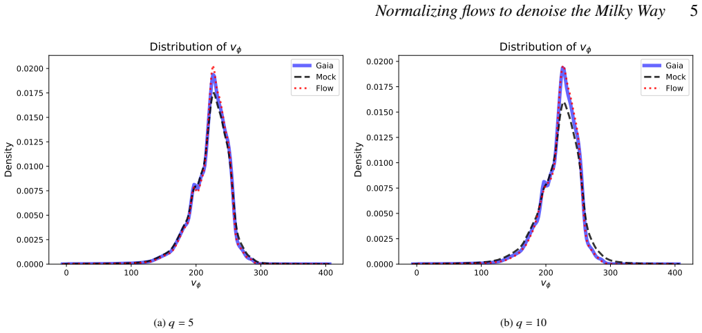
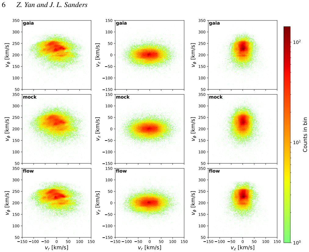
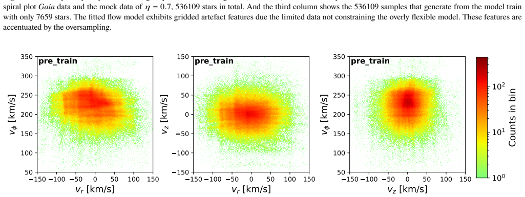
The central claim is that a rational-quadratic-spline autoregressive normalizing flow, trained to maximize the mean of the flow density at importance-sampled points from each star's known uncertainty, approximates the deconvolved 6D phase-space distribution of Gaia-like data. The fitted model, not the corrupted mock sample, reproduces the original solar-neighbourhood Gaia distribution in 1D and 6D projections, sharpening the boundaries of the Hercules stream arches at $v_\phi \approx 200$ km/s and enhancing the phase spiral in $(z, v_z)$. The fidelity degrades gracefully with added noise: at $q=10$ the model still removes noise in the Galactic plane and recovers the strongest kinematic boundaries, although it no longer resolves the substructure of the Hercules stream. The paper also shows that excess spline flexibility with small training sets produces gridded artefacts, and that the method outperforms XDGMM on test loss and visual feature recovery.
Load-bearing premise
The load-bearing premise is that evaluating the flow density at noise-sample points carried into the fitting coordinates, without including the Jacobian determinant of that change of variables, still yields a training objective whose optimum matches the true noise-free density; the paper does not quantify how large this bias is.
Editorial extensions
If this is right
- The method can be applied to Gaia samples beyond the solar neighbourhood, where reported uncertainties are several times larger, to search for moving groups and phase-spiral structure in the outer disc and halo.
- Denoised flow densities provide a noise-free surrogate for direct comparison with dynamical models of bar, spiral, and vertical-resonance features.
- Projecting the denoised flow into action–angle space avoids the artificial features that arise when applying non-linear coordinate transforms directly to noisy data.
- The two-stage importance-sampling training protocol can be carried over to other stellar surveys that supply per-star Gaussian uncertainties, without changing the core algorithm.
- A trained flow acts as a compact, resamplable summary of a survey, enabling lightweight sharing and comparison of Milky Way data products.
Reading between the lines
- Since the loss in Eq. (4) omits the Jacobian of the observable-to-Galactocentric transformation, its bias should grow with distance or with stars on fast orbits; multiplying each importance sample by the local Jacobian would make the loss an unbiased estimator of the marginal likelihood and is the most direct correction to test.
- The paper assumes the reported Gaia uncertainties are exact; injecting deliberately mismatched noise (for example, 20 percent over- or under-estimated errors) and measuring the contrast of the recovered phase spiral would quantify how sensitive the method is to noise-model misspecification.
- A natural extension is to let the number of importance samples $K$ scale with per-star uncertainty, so tiny-error stars contribute few samples and high-error stars contribute many; the paper notes this is possible but does not test it.
- For halo applications the selection function cannot be separated from the noise model; coupling the denoising flow with a selection-function model would be needed before the method is used far from the solar neighbourhood.
Editorial analysis
A structured set of objections, weighed in public.
Referee Report
Summary. The paper proposes a normalizing-flow method for denoising density estimation of stellar survey data with heteroscedastic uncertainties, and demonstrates it on Gaia DR3 RVS data in a local solar-neighborhood volume. The method trains an autoregressive rational-quadratic-spline flow in Galactocentric coordinates using a Monte Carlo importance-sampling loss: for each star, noise samples are drawn in observable space, transformed to Galactocentric coordinates, and the flow density is averaged over them. The authors validate on mock datasets created by inflating the reported Gaia uncertainties by factors q=5 and q=10, comparing against a no-deconvolution baseline, a ground-truth flow fitted to the original Gaia sample, and extreme deconvolution (XDGMM). They report qualitative recovery of the Hercules stream and the phase spiral, plus quantitative test-loss comparisons and a study of hyperparameters K, B, and training-set size.
Significance. If the training objective is correct, the method is a useful advance: it offers a flexible, non-Gaussian alternative to XDGMM for heteroscedastic noise, and the demonstration on real Gaia data with publicly available code is a valuable proof of concept. The paper is appropriately framed as a proof of principle, includes a detailed hyperparameter analysis, and credits the limitations of treating the already-noisy Gaia sample as ground truth. However, the central training objective as implemented is not the convolution likelihood, because the Jacobian of the observable-to-Galactocentric transformation is omitted from the importance-sampling estimator. Until that is corrected and the main figures are reproduced with the corrected loss, the quantitative and qualitative claims must be treated with caution.
major comments (2)
- [Section 3.1 and Algorithm 1; Eq. (4)] The Monte Carlo estimator in Eq. (4) does not compute the convolution likelihood in Galactocentric coordinates. For a flow density P_NF(v_gc), the likelihood of an observation w_i in observable space is p(w_i) = ∫ P_NF(v_gc) p_n(w_i - T^{-1}(v_gc)) dv_gc, where T is the observable-to-Galactocentric map. Sampling v_obs ~ N(w_i, Σ_i) and averaging P_NF(T(v_obs)) gives an estimator of ∫ P_NF(v_gc) p_n(w_i - T^{-1}(v_gc)) |det J_{T^{-1}}(v_gc)| dv_gc, which contains an extra Jacobian factor. The unbiased estimator instead requires weighting each sample by |det J_T(v_obs)| (equivalently dividing by |det J_{T^{-1}}(v_gc)|). Because T includes 1/parallax and proper-motion distance scaling, the Jacobian varies across the sample and across noise realizations for a single star, so the fitted flow is not the true GC-space density. The reported recovery of the Hercules stream (Fig. 2) and phase spiral (Fig. 3) could therefore be shaped by this misspecified objective rather than by genuine deconvolution. I request that the authors correct the loss by including the Jacobian determinant, retrain the models, and verify that the qualitative conclusions persist.
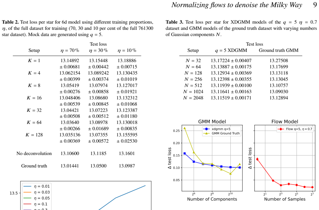
- [Section 3.4; Tables 1 and 2; Fig. 8] The quantitative evaluation selects hyperparameters on the same test set used to report final performance. The number of denoising samples K (Table 1) and the spline bin number B (Fig. 8) are chosen by comparing test losses on the held-out 30% of the Gaia data, and the same test set is then used for the benchmarks and the XDGMM comparison. This makes the reported test losses optimistic and means that the comparisons between configurations are not independent. I recommend introducing a separate validation split for hyperparameter selection and reporting test losses on a final untouched split, or explicitly stating that the quoted values are validation-selected and should be interpreted as upper bounds on performance.
minor comments (5)
- [Section 2.1 and Algorithm 1] The notation in Eq. (3) is ambiguous: it writes the expectation as E_{v∼p_n_i(w_i−v)}[P_NF(v)], but the samples are drawn in observable space and then transformed to Galactocentric coordinates before evaluating P_NF. Please make this explicit in the equations, since the correct treatment of the coordinate change is essential to the method.
- [Section 3.1, Eq. (6)] The quality cut is written as error_over_parallax > 0.5, which selects stars with relative parallax errors greater than 50% and contradicts the description of a high-quality local sample. This is almost certainly a typo for '< 0.5'. Please correct it, as the cut defines the dataset used in all experiments.
- [Table 1] Some entries lack standard deviations: the q=10 column is reported without error bars, and the Ground truth row has no uncertainty. Since these values are used to support the denoising claims, please report run-to-run uncertainties for all configurations.
- [Section 3.4.3] The sentence 'These artefacts are irrelative to the sample number K' contains a typo ('irrelative' should be 'irrelevant'), and the figure captions in Figs. 6 and 7 should be reworded for clarity.
- [Section 2.1] The statement that Gaussian deconvolution is 'well-posed' conflicts with the immediately following discussion of Carroll & Hall (1988), which describes logarithmic convergence rates and sensitivity to sharp features. Please reword to avoid the contradiction, e.g., by saying the problem is well-posed in the strict sense of unique identifiability but severely ill-conditioned in practice.
Circularity Check
No significant circularity: the denoising loss is a Monte Carlo convolution likelihood and the validation uses held-out data with external baselines.
full rationale
The paper's derivation chain is self-contained. Eq. (4) is a Monte Carlo estimate of the convolution in Eq. (2): sampling v from the noise kernel p_ni(w_i - v) and averaging P_NF(v) estimates (P_NF * p_ni)(w_i), so maximizing this loss is a legitimate deconvolution objective rather than a quantity defined in terms of the claimed noise-free density. The claimed denoising results are then tested on a held-out 30% of the original Gaia sample, with the 'ground truth' flow fitted only on the training split, and are compared against an external XDGMM baseline. Hyperparameters (K, B) are chosen via cross-validated test loss, not by fitting the reported substructure recovery. There are no load-bearing self-citations and no known result is merely renamed. The omission of a Jacobian determinant when moving from observable to Galactocentric coordinates in Algorithm 1/Eq. (4) is a potential bias in what density the flow actually fits, but it is a correctness/approximation concern, not circularity: the optimized density is not equivalent to its input by construction. The Appendix A2 caveat that multiple deconvolved distributions are consistent with finite noisy data is an identifiability/uncertainty statement, not circular reasoning.
Assumptions & free parameters
free parameters (3)
- denoising samples per star K =
128
- spline bin number B =
32
- noise amplification factor q =
5 and 10
assumptions (4)
- domain assumption The noise distributions p_{n_i} are known exactly for every star.
- ad hoc to paper The observable-to-Galactocentric transformation can be applied to noise samples without a Jacobian correction in the importance-sampling loss.
- domain assumption The normalizing flow is sufficiently expressive to represent the true underlying distribution.
- domain assumption Selection effects and completeness can be ignored for the mock-data test.
Cite this review
Pith. "Pith review of Denoising Milky Way stellar survey data with normalizing flow models." pith.science (2026). https://pith.science/paper/5MGNYO7L
@misc{pith2026250516553,
  author       = {Pith},
  title        = {Pith review of: Denoising Milky Way stellar survey data with normalizing flow models},
  year         = {2026},
  howpublished = {\url{https://pith.science/paper/5MGNYO7L}},
  note         = {Machine review of arXiv:2505.16553}
}
read the original abstract
The Gaia dataset has revealed many intricate Milky Way substructures in exquisite detail, including moving groups and the phase spiral. Precise characterisation of these features and detailed comparisons to theoretical models require engaging with Gaia's heteroscedastic noise model, particularly in more distant parts of the Galactic disc and halo. We propose a general, novel machine-learning approach using normalizing flows for denoising density estimation, with particular focus on density estimation from stellar survey data such as that from Gaia. Normalizing flows transform a simple base distribution into a complex target distribution through bijective transformations resulting in a highly expressive and flexible model. The denoising is performed using importance sampling. We demonstrate that this general procedure works excellently on Gaia data by reconstructing detailed local velocity distributions artificially corrupted with noise. For example, we show the multiple branches of the Hercules stream and the phase-space spiral can both be well captured by our model. We discuss hyperparameter choice to optimally recover substructure and compare our approach to extreme deconvolution. The model therefore promises to be a robust tool for studying the Milky Way's kinematics in Galactic locations where the noise from Gaia is significant.
Figures

Figures from the paper (6 more)




Forward citations
Cited by 1 Pith paper
-
Deep Potential: Recovering the gravitational potential and local pattern speed in the solar neighborhood with GDR3 using normalizing flows
Using normalizing flows and a neural network on Gaia DR3 data, the authors recover a local pattern speed of 28.2 km/s/kpc and a total matter density of 0.086 solar masses per cubic parsec within 1 kpc of the Sun.
Reference graph
Works this paper leans on
-
[1]
W., Leistedt B., Price-Whelan A
Anderson L., Hogg D. W., Leistedt B., Price-Whelan A. M., Bovy J., 2018, @doi [ ] 10.3847/1538-3881/aad7bf , https://ui.adsabs.harvard.edu/abs/2018AJ....156..145A 156, 145
-
[2]
Antoja T., et al., 2018, @doi [ ] 10.1038/s41586-018-0510-7 , https://ui.adsabs.harvard.edu/abs/2018Natur.561..360A 561, 360
-
[3]
Antoja T., Ramos P., Garc \' a-Conde B., Bernet M., Laporte C. F. P., Katz D., 2023, @doi [ ] 10.1051/0004-6361/202245518 , https://ui.adsabs.harvard.edu/abs/2023A&A...673A.115A 673, A115
-
[4]
Ascasibar Y., Binney J., 2005, @doi [ ] 10.1111/j.1365-2966.2004.08480.x , https://ui.adsabs.harvard.edu/abs/2005MNRAS.356..872A 356, 872
arXiv 2005
-
[5]
Astropy Collaboration et al., 2022, @doi [ ] 10.3847/1538-4357/ac7c74 , https://ui.adsabs.harvard.edu/abs/2022ApJ...935..167A 935, 167
-
[6]
Bovy J., Hogg D. W., Roweis S. T., 2011, @doi [Annals of Applied Statistics] 10.1214/10-AOAS439 , https://ui.adsabs.harvard.edu/abs/2011AnApS...5.1657B 5, 1657
-
[7]
J., Hall P., 1988, Journal of the American Statistical Association, 83, 1184
Carroll R. J., Hall P., 1988, Journal of the American Statistical Association, 83, 1184
work page 1988
-
[8]
Ciuca I., Ting Y.-S., 2022, in Machine Learning for Astrophysics. p. 17 ( @eprint arXiv 2207.02785 ), @doi 10.48550/arXiv.2207.02785
work page Pith review arXiv doi:10.48550/arxiv.2207.02785 2022
Show all 49 references
-
[9]
Cropper M., et al., 2018, @doi [ ] 10.1051/0004-6361/201832763 , https://ui.adsabs.harvard.edu/abs/2018A&A...616A...5C 616, A5
2018 doi
-
[10]
Darvish B., Mobasher B., Sobral D., Scoville N., Aragon-Calvo M., 2015, @doi [ ] 10.1088/0004-637X/805/2/121 , https://ui.adsabs.harvard.edu/abs/2015ApJ...805..121D 805, 121
2015 doi
- [11]
-
[12]
A., Bovy J., Myers A
DiPompeo M. A., Bovy J., Myers A. D., Lang D., 2015, @doi [ ] 10.1093/mnras/stv1562 , https://ui.adsabs.harvard.edu/abs/2015MNRAS.452.3124D 452, 3124
2015 doi
- [13]
-
[14]
A., Yu Y., Murray I., 2020, @doi [arXiv e-prints] 10.48550/arXiv.2006.09396 , https://ui.adsabs.harvard.edu/abs/2020arXiv200609396D p
Dockhorn T., Ritchie J. A., Yu Y., Murray I., 2020, @doi [arXiv e-prints] 10.48550/arXiv.2006.09396 , https://ui.adsabs.harvard.edu/abs/2020arXiv200609396D p. arXiv:2006.09396
- [15]
-
[16]
Fan J., 1991, @doi [The Annals of Statistics] 10.1214/aos/1176348248 , 19, 1257
1991
-
[17]
J., Buddelmeijer H., Trager S
Ferdosi B. J., Buddelmeijer H., Trager S. C., Wilkinson M. H. F., Roerdink J. B. T. M., 2011, @doi [ ] 10.1051/0004-6361/201116878 , https://ui.adsabs.harvard.edu/abs/2011A&A...531A.114F 531, A114
2011 doi
-
[18]
Gaia Collaboration et al., 2016, @doi [ ] 10.1051/0004-6361/201629272 , https://ui.adsabs.harvard.edu/abs/2016A&A...595A...1G 595, A1
2016 doi
-
[19]
Gaia Collaboration et al., 2018, @doi [ ] 10.1051/0004-6361/201832865 , https://ui.adsabs.harvard.edu/abs/2018A&A...616A..11G 616, A11
2018 doi
-
[20]
Gaia Collaboration et al., 2023a, @doi [ ] 10.1051/0004-6361/202243940 , https://ui.adsabs.harvard.edu/abs/2023A&A...674A...1G 674, A1
-
[21]
Gaia Collaboration et al., 2023b, @doi [ ] 10.1051/0004-6361/202243797 , https://ui.adsabs.harvard.edu/abs/2023A&A...674A..37G 674, A37
- [22]
- [23]
-
[24]
M., Ting Y.-S., Kamdar H., 2023, @doi [ ] 10.3847/1538-4357/aca3a7 , https://ui.adsabs.harvard.edu/abs/2023ApJ...942...26G 942, 26
Green G. M., Ting Y.-S., Kamdar H., 2023, @doi [ ] 10.3847/1538-4357/aca3a7 , https://ui.adsabs.harvard.edu/abs/2023ApJ...942...26G 942, 26
2023 doi
-
[25]
R., et al., 2020, @doi [ ] 10.1038/s41586-020-2649-2 , https://ui.adsabs.harvard.edu/abs/2020Natur.585..357H 585, 357
Harris C. R., et al., 2020, @doi [ ] 10.1038/s41586-020-2649-2 , https://ui.adsabs.harvard.edu/abs/2020Natur.585..357H 585, 357
2020 doi
-
[26]
D., 2007, @doi [Computing in Science and Engineering] 10.1109/MCSE.2007.55 , https://ui.adsabs.harvard.edu/abs/2007CSE.....9...90H 9, 90
Hunter J. D., 2007, @doi [Computing in Science and Engineering] 10.1109/MCSE.2007.55 , https://ui.adsabs.harvard.edu/abs/2007CSE.....9...90H 9, 90
2007 doi
-
[27]
M., Ghosh S., 2024, @doi [ ] 10.1093/mnras/stae011 , https://ui.adsabs.harvard.edu/abs/2024MNRAS.52712284K 527, 12284
Kalda T., Green G. M., Ghosh S., 2024, @doi [ ] 10.1093/mnras/stae011 , https://ui.adsabs.harvard.edu/abs/2024MNRAS.52712284K 527, 12284
2024 doi
-
[28]
F., Schindler J.-T., Tamanas J., Nanni R., 2024, @doi [arXiv e-prints] 10.48550/arXiv.2412.03029 , https://ui.adsabs.harvard.edu/abs/2024arXiv241203029K p
Kang Y., Hennawi J. F., Schindler J.-T., Tamanas J., Nanni R., 2024, @doi [arXiv e-prints] 10.48550/arXiv.2412.03029 , https://ui.adsabs.harvard.edu/abs/2024arXiv241203029K p. arXiv:2412.03029
- [29]
-
[30]
P., Dhariwal P., 2018, @doi [arXiv e-prints] 10.48550/arXiv.1807.03039 , https://ui.adsabs.harvard.edu/abs/2018arXiv180703039K p
Kingma D. P., Dhariwal P., 2018, @doi [arXiv e-prints] 10.48550/arXiv.1807.03039 , https://ui.adsabs.harvard.edu/abs/2018arXiv180703039K p. arXiv:1807.03039
- [31]
-
[32]
M., Kraus A
Krolikowski D. M., Kraus A. L., Rizzuto A. C., 2021, @doi [ ] 10.3847/1538-3881/ac0632 , https://ui.adsabs.harvard.edu/abs/2021AJ....162..110K 162, 110
2021 doi
-
[33]
S., 2024, @doi [arXiv e-prints] 10.48550/arXiv.2408.11414 , https://ui.adsabs.harvard.edu/abs/2024arXiv240811414L p
Li Z., Han J., Wang W., Qian Y.-Z., Li Q., Jing Y., Li T. S., 2024, @doi [arXiv e-prints] 10.48550/arXiv.2408.11414 , https://ui.adsabs.harvard.edu/abs/2024arXiv240811414L p. arXiv:2408.11414
-
[34]
H., Putney E., Buckley M
Lim S. H., Putney E., Buckley M. R., Shih D., 2025, @doi [ ] 10.1088/1475-7516/2025/01/021 , https://ui.adsabs.harvard.edu/abs/2025JCAP...01..021L 2025, 021
2025 doi
- [35]
-
[36]
C., Figueras F., Roca-F \`a brega S., Luri X., 2019, @doi [ ] 10.1051/0004-6361/201935105 , https://ui.adsabs.harvard.edu/abs/2019A&A...624L...1M 624, L1
Mor R., Robin A. C., Figueras F., Roca-F \`a brega S., Luri X., 2019, @doi [ ] 10.1051/0004-6361/201935105 , https://ui.adsabs.harvard.edu/abs/2019A&A...624L...1M 624, L1
2019 doi
- [37]
- [38]
- [39]
- [40]
-
[41]
Poggio E., et al., 2021, @doi [ ] 10.1051/0004-6361/202140687 , https://ui.adsabs.harvard.edu/abs/2021A&A...651A.104P 651, A104
2021 doi
-
[42]
Ramos P., et al., 2022, @doi [ ] 10.1051/0004-6361/202142830 , https://ui.adsabs.harvard.edu/abs/2022A&A...666A..64R 666, A64
2022 doi
- [43]
-
[44]
Rozet F., Divo F., Schnake S., 2024, probabilists/zuko: Zuko 1.1.0 , @doi 10.5281/zenodo.7625672
2024 doi
-
[45]
Sch \"o nrich R., Dehnen W., 2018, @doi [ ] 10.1093/mnras/sty1256 , https://ui.adsabs.harvard.edu/abs/2018MNRAS.478.3809S 478, 3809
2018 doi
-
[46]
Sharma S., Steinmetz M., 2006, @doi [ ] 10.1111/j.1365-2966.2006.11043.x , https://ui.adsabs.harvard.edu/abs/2006MNRAS.373.1293S 373, 1293
2006
- [47]
- [48]
-
[49]
write newline
" write newline "" before.all 'output.state := FUNCTION fin.entry write newline FUNCTION new.block output.state before.all = 'skip after.block 'output.state := if FUNCTION new.sentence output.state after.block = 'skip output.state before.all = 'skip after.sentence 'output.stat...
Reviewed August 7, 2026 · model on record in the stance chip above.
Discussion (0). Continue with ORCID to comment.