REVIEW 4 major objections 5 minor 57 references
Approach to Finding a Robust Deep Learning Model
T0 review · 4 major / 5 minor · reviewed 2026-08-07 · deepseek-v4-flash
Pith's one-line read A model is robust if its instances — retrained on different samples and weight initializations — land close together in test loss, and the paper's selection algorithm finds such models while training far fewer instances than exhaustive…
desk verdict Solid empirical study of small CNN robustness on calorimeter data, but the selection algorithm prunes by mean loss, so the headline claim that it finds the most robust models is not supported as reported. read the letter →
The pith
A machine-rendered reading of the paper's core claim, the machinery that carries it, and where it could break.
The reading
What carries the argument
The carrying mechanism is the instance-loss distribution: train many instances of a candidate model, each on a randomly drawn training sample with randomly initialized weights, collect the test losses, and read robustness off their spread. For selection, the paper wraps this in Algorithm 1: starting from the full set of models, train one new instance per model per step, update a running robustness value (here the mean loss), and after k steps drop models whose value misses the selection criterion, continuing until one model remains. All losses are generated under a fixed early stopping rule — every instance trains to at least epoch 100 and stops when the maximum loss in the previous 30 epochs exceeds the minimum loss in the previous 30 epochs by 10% — and for the final comparison, 50 instances per surviving model are used to fix the robustness estimate.
What would settle it
A concrete check: train 1,000 instances of a fixed configuration on a fixed training sample under the paper's early-stopping rule, then train another 1,000 to a fixed 500 epochs with no early stopping; if the two test-loss spreads differ materially, the stopping rule, not the model, is shaping the robustness measurement.
Extended reading notes
Core claim
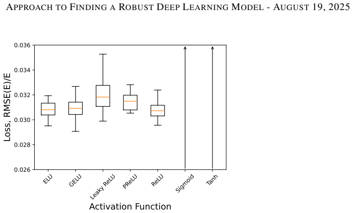
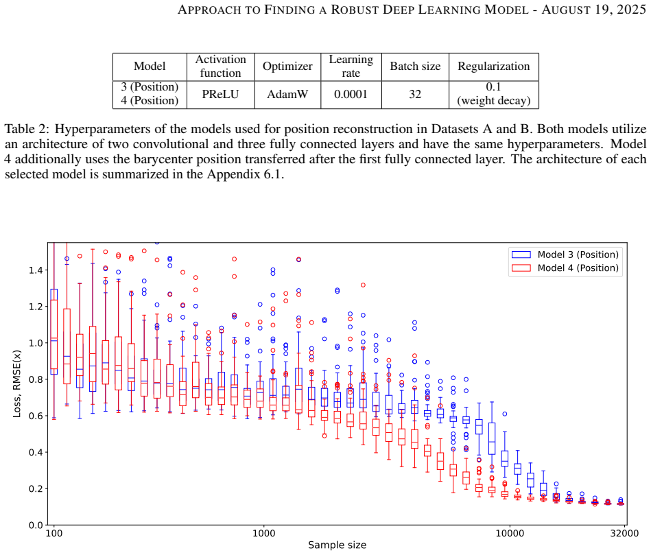
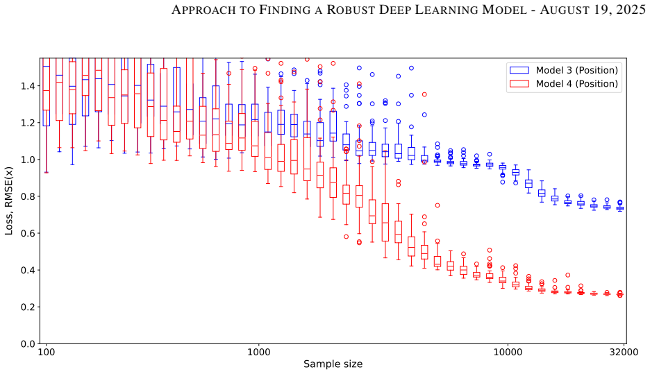
On the paper's own terms, the central discovery is that repeated-seed loss variability is a usable, model-agnostic measure of robustness. A model is called robust if its instances — identical architecture and hyperparameters, trained from different random weight initializations and different fixed-size training samples from one population — yield test losses close to each other, with closeness quantified by a chosen statistical criterion over the instance loss set. The corresponding selection algorithm prunes candidate models by their mean loss over successively trained instances, so that after 12 iterations over 6,912 energy-reconstruction configurations it selected a two-convolutional, two-fully-connected model with ReLU/NAdam and a version augmented with the sum of cell energies; on the position task it selected PReLU/AdamW models with and without a barycenter feature. The paper reports that the selected models had the best convergence and smallest loss variability among the configurations considered, that the energy model with inductive bias reaches robust behavior on Dataset A with about 2,000 training examples while the raw-feature model needs about 18,000, and that for the raw-feature model sampling randomness dominates initialization randomness while for the inductive-bias model the ordering is weakly reversed.
Load-bearing premise
Every robustness result depends on the early stopping rule — train to at least 100 epochs and stop when the worst loss in a 30-epoch window is 10% above the best loss in that window — actually identifying converged models, because if it stops too early or too late, the measured spread of test losses reflects the stopping rule rather than the model.
Editorial extensions
If this is right
- Any machine learning model can be assessed for robustness by training a set of instances and measuring the spread of test losses, without changing the model itself.
- The selection algorithm cuts the cost of finding a robust model: 41,567 model/instance trainings instead of 345,600 for an exhaustive search with the same 50-instance guarantee.
- Adding a physically motivated inductive bias (sum of energy deposits, or barycenter position) lowers the sample size at which a model becomes robust and speeds convergence, without sacrificing the robustness level.
- For the raw-feature energy model, random sampling of the training set affects loss variability more than weight initialization; for the inductive-bias model, initialization matters slightly more, but the gap is smaller.
- The approach quantifies the closeness of performance across instances, which is the property a fault-tolerant automated-training pipeline needs before a model is passed to the next optimization step.
Reading between the lines
- A testable extension the paper leaves implicit: the same instance-loss spread could be computed on a shifted population (train on Dataset A, test on Dataset B) to turn the robustness measure into a distribution-shift sensitivity index; the paper only uses Dataset B as a final generalization check.
- The cost saving of Algorithm 1 rests on an ordering assumption — that mean loss over a few instances ranks models like mean loss over many. A reader could verify this by running the algorithm's early steps on a random subset of configurations and comparing the pruned ranking with the full 50-instance ranking.
- The early stopping rule's 10-percent hysteresis threshold is a free parameter; varying it would show how much of the measured loss spread is intrinsic to the model and how much is an artifact of when training is cut off.
Editorial analysis
A structured set of objections, weighed in public.
Referee Report
Summary. The paper proposes an operational definition of model robustness: a model is robust if its independently trained instances (differing only in random weight initialization and training-sample draw) produce close test losses. It also proposes a meta-algorithm (Algorithm 1) that iteratively trains a small number of instances per model and prunes unpromising models using a selection criterion, intended to identify robust models among top-performing ones. The method is demonstrated on two simulated calorimeter regression tasks (energy and position reconstruction) over a space of 6,912 small CNN models per task. For the selected models, the paper studies minimum training sample size, the relative contributions of sampling and weight initialization, inductive bias, and compares with two NAS-found models.
Significance. If the approach works as claimed, it would provide a practical, computationally efficient way to select robust deep-learning models for AutoML and fault-tolerant systems, where repeated-seed loss variability is a meaningful reliability criterion. The paper's strengths include a clear and operational definition of robustness, an unusually large training campaign (41,567 trained model instances), the use of well-defined simulated datasets with fixed train/test partitions, and a comparison against NAS baselines. The definition of robustness as across-instance loss closeness is reasonable and could be useful beyond the specific architectures studied. However, the central claim that the proposed algorithm actually selects the most robust models is not supported by the reported experiments, because the selection criterion is mean loss rather than a spread statistic, and the spread is measured only for the surviving models.
major comments (4)
- [Section 3.10 and Algorithm 1] The robustness definition in Section 3 is explicitly about closeness of test losses across independently trained instances, i.e., a spread statistic. Yet Algorithm 1 is run with 'mean loss as the selection criterion' (Section 3.10, paragraph 4). Mean loss is a location statistic: it ranks average performance, not the closeness of instance losses. Under mean-loss pruning, a low-mean/high-variance model is indistinguishable from a low-mean/low-variance model, and a high-mean/low-variance model is discarded. The paper only computes the 50-instance spread for the two surviving models; it never computes spread for pruned models. Therefore the Conclusion's statement that these models have 'the smallest loss variability among the 2×6,912 models' is not a reported result. Please either measure the spread for a random sample of pruned models to validate the pruning, change the selection criterion to a spread-based statistic, or substantially weaken the claim.
- [Section 3.10, computational saving] The claimed computational saving (41,567 vs 345,600 trained instances) is conditional on the unverified assumption that pruning by one/few instances and by mean loss does not discard models that would have had the smallest final spread. With no evidence about the distribution of spread among pruned models, the saving is not established. A concrete test would be to run the full exhaustive search on a random subset of the 6,912 models, or at least to compute final spreads for a random sample of models discarded in each pruning round.
- [Section 3.7, early stopping] The early stopping rule (all instances trained to at least epoch 100, stop when the max loss in the previous 30 epochs exceeds the min loss in the same window by 10%) uses hand-picked thresholds with no sensitivity analysis. All robustness distributions are computed from models stopped by this rule, so the minimum-sample-size conclusions in Section 4 (e.g., '18,000 (2,000) examples' for Model 1/Model 2) may be artifacts of the stopping heuristic. Please report the distribution of stopping epochs across the 6,912 models, and provide an ablation varying the minimum epoch count, window size, and tolerance to show that the qualitative conclusions are unchanged.
- [Abstract and Section 1, generality claim] The abstract states the approach is 'versatile and applicable to any machine learning model', but the empirical support is limited to small CNNs (up to 24k parameters) on two simulated calorimeter regression tasks from the same generator. The sample-size and initialization studies in Section 4 also use only these two tasks. Please temper the generality claim to the demonstrated scope, or add a second, unrelated benchmark (e.g., an image classification or tabular regression task) to support the claimed versatility.
minor comments (5)
- [Section 1, first paragraph of the robustness discussion] There is a typo: 'the authors of the paper [23] discuss ... and propose several additional several additional data sets' should read 'several additional data sets'.
- [Figures 4 and 5 captions] The captions of Figures 4 and 5 state that Model 2 uses the sum of energies transferred after the first convolution layer, but the text in Section 3.8 and the architecture appendix consistently say 'after the first fully connected layer'. Please correct the captions.
- [Figure 13 and Figure 14 captions] Figures 13 and 14 have identical captions; the zoomed/re-binned version should be identified as such (as mentioned in the body text but not in the caption).
- [Section 3.10, sample size formula] The formula for the ith training sample size, '2,000 · 10^(−1.18 + i·2.38/44)', would be clearer with a brief explanation of the chosen range and endpoints, and the use of a comma as a thousands separator in the displayed formula is confusing.
- [Section 4.1, paragraph on Figure 4] The sentence 'for almost all instances of Model 1 shows a higher value of the loss' is grammatically incomplete; it should read 'for almost all instances, Model 1 shows a higher loss value'.
Circularity Check
No significant circularity; the mean-loss pruning gap is an evidentiary overclaim, not a circular reduction.
full rationale
Walking the claimed derivation chain, no step is equivalent to its own input by construction. Robustness is defined operationally as a statistical measure (variability) of test losses over independently trained instances, and the model selection algorithm is a separate heuristic that prunes by mean loss. The 50-instance robustness measurements for the two surviving models are new empirical measurements, not fitted values renamed as predictions. The conclusion that the selected models have the 'smallest loss variability among the 2×6,912 models' is not directly established, because spread was only computed for the survivors while pruning was based on mean loss; however, this is an evidentiary gap or overclaim, not a circular argument. The self-citations ([10], [33]) are contextual or provide an external XGBoost baseline from prior work; they are not load-bearing for the robustness claim. The early-stopping rule is a fixed heuristic applied uniformly to all instances and does not encode the target loss-variability conclusion. Therefore the paper's core derivation remains self-contained and no specific reduction to its inputs can be exhibited.
Assumptions & free parameters
free parameters (6)
- Early stopping minimum epoch count =
100 epochs
- Early stopping window size =
30 epochs
- Early stopping relative tolerance =
10%
- Initial model-selection pruning threshold =
baseline loss + 20%
- Per-round discard fraction =
half of remaining models
- Number of instances per model k =
10, 50, or 1000 depending on experiment
assumptions (6)
- domain assumption The random 0.5/0.5 split of the 500,000-sample dataset, with training subsamples bootstrapped from the first half and testing on the second half, yields training and test sets from the same population with similarly distributed outliers.
- domain assumption RMSE(E)/E is an appropriate loss to equalize energy-resolution stochasticity across energies.
- standard math He initialization is appropriate for all models.
- ad hoc to paper The early stopping rule identifies convergence and explosive loss behavior.
- ad hoc to paper Pruning by mean loss, with an initial baseline+20% cutoff and half-discard per round, preserves the most robust models.
- domain assumption The GEANT4 simulation of the Shashlik calorimeter is a faithful proxy for real calorimeter response.
Cite this review
Pith. "Pith review of Approach to Finding a Robust Deep Learning Model." pith.science (2026). https://pith.science/paper/CVYRJWUC
@misc{pith2026250517254,
  author       = {Pith},
  title        = {Pith review of: Approach to Finding a Robust Deep Learning Model},
  year         = {2026},
  howpublished = {\url{https://pith.science/paper/CVYRJWUC}},
  note         = {Machine review of arXiv:2505.17254}
}
read the original abstract
The rapid development of machine learning (ML) and artificial intelligence (AI) applications requires the training of large numbers of models. This growing demand highlights the importance of training models without human supervision, while ensuring that their predictions are reliable. In response to this need, we propose a novel approach for determining model robustness. This approach, supplemented with a proposed model selection algorithm designed as a meta-algorithm, is versatile and applicable to any machine learning model, provided that it is appropriate for the task at hand. This study demonstrates the application of our approach to evaluate the robustness of deep learning models. To this end, we study small models composed of a few convolutional and fully connected layers, using common optimizers due to their ease of interpretation and computational efficiency. Within this framework, we address the influence of training sample size, model weight initialization, and inductive bias on the robustness of deep learning models.
Figures


Figures from the paper (15 more)





Reference graph
Works this paper leans on
-
[1]
Approximation by superpositions of a sigmoidal function
George Cybenko. Approximation by superpositions of a sigmoidal function. Mathematics of control, signals and systems, 2(4):303–314, 1989
1989
-
[2]
Approximating continuous functions by relu nets of minimal width
Boris Hanin and Mark Sellke. Approximating continuous functions by relu nets of minimal width. arXiv preprint arXiv:1710.11278, 2017
arXiv 2017
-
[3]
Speeding up the hyperparameter optimization of deep convolutional neural networks
Tobias Hinz, Nicolás Navarro-Guerrero, Sven Magg, and Stefan Wermter. Speeding up the hyperparameter optimization of deep convolutional neural networks. International Journal of Computational Intelligence and Applications, 17(02):1850008, 2018
work page 2018
-
[4]
A comprehensive survey of neural architecture search: Challenges and solutions
Pengzhen Ren, Yun Xiao, Xiaojun Chang, Po-Yao Huang, Zhihui Li, Xiaojiang Chen, and Xin Wang. A comprehensive survey of neural architecture search: Challenges and solutions. ACM Computing Surveys (CSUR), 54(4):1–34, 2021
work page 2021
-
[5]
Neural architecture search benchmarks: Insights and survey
Krishna Teja Chitty-Venkata, Murali Emani, Venkatram Vishwanath, and Arun K Somani. Neural architecture search benchmarks: Insights and survey. IEEE Access, 11:25217–25236, 2023
work page 2023
-
[6]
Nas-bench-101: Towards reproducible neural architecture search
Chris Ying, Aaron Klein, Eric Christiansen, Esteban Real, Kevin Murphy, and Frank Hutter. Nas-bench-101: Towards reproducible neural architecture search. In International conference on machine learning, pages 7105–
-
[7]
Nas-bench-201: Extending the scope of reproducible neural architecture search
Xuanyi Dong and Yi Yang. Nas-bench-201: Extending the scope of reproducible neural architecture search. arXiv preprint arXiv:2001.00326, 2020
arXiv 2001
-
[8]
Nas-bench-nlp: neural architecture search benchmark for natural language processing
Nikita Klyuchnikov, Ilya Trofimov, Ekaterina Artemova, Mikhail Salnikov, Maxim Fedorov, Alexander Filippov, and Evgeny Burnaev. Nas-bench-nlp: neural architecture search benchmark for natural language processing. IEEE Access, 10:45736–45747, 2022. 24 APPROACH TO FINDING A ROBUST DEEP LEARNING MODEL - AUGUST 19, 2025
work page 2022
Show all 57 references
-
[9]
Automl: A survey of the state-of-the-art
Xin He, Kaiyong Zhao, and Xiaowen Chu. Automl: A survey of the state-of-the-art. Knowledge-based systems, 212:106622, 2021
2021
-
[10]
Toward the end-to-end optimization of particle physics instruments with differentiable programming
Tommaso Dorigo, Andrea Giammanco, Pietro Vischia, Max Aehle, Mateusz Bawaj, Alexey Boldyrev, Pablo de Castro Manzano, Denis Derkach, Julien Donini, Auralee Edelen, et al. Toward the end-to-end optimization of particle physics instruments with differentiable programming. Review...
2023
-
[11]
Huber and E.M
P.J. Huber and E.M. Ronchetti. Robust Statistics. Wiley Series in Probability and Statistics. Wiley, 2011
2011
-
[12]
Training set size requirements for the classification of a specific class
Giles M Foody, Ajay Mathur, Carolina Sanchez-Hernandez, and Doreen S Boyd. Training set size requirements for the classification of a specific class. Remote Sensing of Environment, 104(1):1–14, 2006
2006
-
[13]
Riesz networks: Scale-invariant neural networks in a single forward pass
Tin Barisin, Katja Schladitz, and Claudia Redenbach. Riesz networks: Scale-invariant neural networks in a single forward pass. Journal of Mathematical Imaging and Vision, pages 1–25, 2024
2024
-
[14]
An image is worth 16x16 words: Transformers for image recognition at scale
Alexey Dosovitskiy, Lucas Beyer, Alexander Kolesnikov, Dirk Weissenborn, Xiaohua Zhai, Thomas Unterthiner, Mostafa Dehghani, Matthias Minderer, Georg Heigold, Sylvain Gelly, et al. An image is worth 16x16 words: Transformers for image recognition at scale. arXiv preprint arXiv...
2010 arXiv
-
[15]
Delving deep into rectifiers: Surpassing human-level performance on imagenet classification
Kaiming He, Xiangyu Zhang, Shaoqing Ren, and Jian Sun. Delving deep into rectifiers: Surpassing human-level performance on imagenet classification. In Proceedings of the IEEE international conference on computer vision, pages 1026–1034, 2015
2015
-
[16]
Imagenet: A large-scale hierarchical image database
Jia Deng, Wei Dong, Richard Socher, Li-Jia Li, Kai Li, and Li Fei-Fei. Imagenet: A large-scale hierarchical image database. In 2009 IEEE conference on computer vision and pattern recognition, pages 248–255. Ieee, 2009
2009
-
[17]
Robust training and initialization of deep neural networks: An adaptive basis viewpoint
Eric C Cyr, Mamikon A Gulian, Ravi G Patel, Mauro Perego, and Nathaniel A Trask. Robust training and initialization of deep neural networks: An adaptive basis viewpoint. In Mathematical and Scientific Machine Learning, pages 512–536. PMLR, 2020
2020
-
[18]
Deep residual learning for image recognition
Kaiming He, Xiangyu Zhang, Shaoqing Ren, and Jian Sun. Deep residual learning for image recognition. In Proceedings of the IEEE conference on computer vision and pattern recognition, pages 770–778, 2016
2016
-
[19]
Robustness in deep learning: The good (width), the bad (depth), and the ugly (initialization)
Zhenyu Zhu, Fanghui Liu, Grigorios Chrysos, and V olkan Cevher. Robustness in deep learning: The good (width), the bad (depth), and the ugly (initialization). Advances in neural information processing systems, 35:36094–36107, 2022
2022
-
[20]
Double descent demystified: Identifying, interpreting & ablating the sources of a deep learning puzzle
Rylan Schaeffer, Mikail Khona, Zachary Robertson, Akhilan Boopathy, Kateryna Pistunova, Jason W Rocks, Ila Rani Fiete, and Oluwasanmi Koyejo. Double descent demystified: Identifying, interpreting & ablating the sources of a deep learning puzzle. arXiv preprint arXiv:2303.14151, 2023
2023 arXiv
-
[21]
The difficulty of computing stable and accurate neural networks: On the barriers of deep learning and smale’s 18th problem
Matthew J Colbrook, Vegard Antun, and Anders C Hansen. The difficulty of computing stable and accurate neural networks: On the barriers of deep learning and smale’s 18th problem. Proceedings of the National Academy of Sciences, 119(12):e2107151119, 2022
2022
-
[22]
Stable architectures for deep neural networks
Eldad Haber and Lars Ruthotto. Stable architectures for deep neural networks. Inverse problems, 34(1):014004, 2017
2017
-
[23]
The many faces of robustness: A critical analysis of out-of-distribution generalization
Dan Hendrycks, Steven Basart, Norman Mu, Saurav Kadavath, Frank Wang, Evan Dorundo, Rahul Desai, Tyler Zhu, Samyak Parajuli, Mike Guo, et al. The many faces of robustness: A critical analysis of out-of-distribution generalization. In Proceedings of the IEEE/CVF international c...
2021
-
[24]
Inductive biases for deep learning of higher-level cognition
Anirudh Goyal and Yoshua Bengio. Inductive biases for deep learning of higher-level cognition. Proceedings of the Royal Society A, 478(2266):20210068, 2022
2022
-
[25]
Wilds: A benchmark of in-the-wild distribution shifts
Pang Wei Koh, Shiori Sagawa, Henrik Marklund, Sang Michael Xie, Marvin Zhang, Akshay Balsubramani, Weihua Hu, Michihiro Yasunaga, Richard Lanas Phillips, Irena Gao, et al. Wilds: A benchmark of in-the-wild distribution shifts. In International conference on machine learning, p...
2021
-
[26]
Im- proving robustness against common corruptions by covariate shift adaptation
Steffen Schneider, Evgenia Rusak, Luisa Eck, Oliver Bringmann, Wieland Brendel, and Matthias Bethge. Im- proving robustness against common corruptions by covariate shift adaptation. Advances in neural information processing systems, 33:11539–11551, 2020
2020
-
[27]
Recent advances in adversarial training for adversarial robustness
Tao Bai, Jinqi Luo, Jun Zhao, Bihan Wen, and Qian Wang. Recent advances in adversarial training for adversarial robustness. arXiv preprint arXiv:2102.01356, 2021
2021 arXiv
-
[28]
Opportunities and challenges in deep learning adversarial robustness: A survey
Samuel Henrique Silva and Peyman Najafirad. Opportunities and challenges in deep learning adversarial robustness: A survey. arXiv preprint arXiv:2007.00753, 2020
2007 arXiv
-
[29]
Tree-structured parzen estimator: Understanding its algorithm components and their roles for better empirical performance
Shuhei Watanabe. Tree-structured parzen estimator: Understanding its algorithm components and their roles for better empirical performance. arXiv preprint arXiv:2304.11127, 2023. 25 APPROACH TO FINDING A ROBUST DEEP LEARNING MODEL - AUGUST 19, 2025
2023 arXiv
-
[30]
Geant4—a simulation toolkit
Sea Agostinelli, John Allison, K al Amako, John Apostolakis, H Araujo, Pedro Arce, Makoto Asai, D Axen, Swagato Banerjee, GJNI Barrand, et al. Geant4—a simulation toolkit. Nuclear instruments and methods in physics research section A: Accelerators, Spectrometers, Detectors and...
2003
-
[31]
Design and construction of electromagnetic calorimeter for lhcb experiment
S Barsuk, V Kochetkov, A Soldatov, S Malyshev, A Golutvin, I Korolko, E Tarkovski, V Mayatski, and V Yu Rusinov. Design and construction of electromagnetic calorimeter for lhcb experiment. Technical report, CERN- LHCb-2000-043, 2000
2000
-
[32]
The lhcb detector at the lhc
A Augusto Alves Jr, LM Andrade Filho, AF Barbosa, I Bediaga, G Cernicchiaro, G Guerrer, HP Lima Jr, AA Machado, J Magnin, F Marujo, et al. The lhcb detector at the lhc. Journal of instrumentation, 3(08):S08005, 2008
2008
-
[33]
Ml-assisted versatile approach to calorimeter r&d
Alexey Boldyrev, Denis Derkach, Fedor Ratnikov, and Andrey Shevelev. Ml-assisted versatile approach to calorimeter r&d. Journal of Instrumentation, 15(09):C09030, 2020
2020
-
[34]
Root—an object oriented data analysis framework
Rene Brun and Fons Rademakers. Root—an object oriented data analysis framework. Nuclear instruments and methods in physics research section A: accelerators, spectrometers, detectors and associated equipment , 389(1-2):81–86, 1997
1997
-
[35]
Jim Pivarski, Henry Schreiner, Angus Hollands, Pratyush Das, Kush Kothari, Aryan Roy, Jerry Ling, Nicholas Smith, Chris Burr, and Giordon Stark. Uproot. Zenodo, 2017
2017
-
[36]
Pytorch: An imperative style, high-performance deep learning library
Adam Paszke, Sam Gross, Francisco Massa, Adam Lerer, James Bradbury, Gregory Chanan, Trevor Killeen, Zeming Lin, Natalia Gimelshein, Luca Antiga, et al. Pytorch: An imperative style, high-performance deep learning library. Advances in neural information processing systems, 32, 2019
2019
-
[37]
A simple method of shower localization and identification in laterally segmented calorimeters
TC Awes, FE Obenshain, F Plasil, Surender Saini, SP Sorensen, and GR Young. A simple method of shower localization and identification in laterally segmented calorimeters. Nuclear Instruments and Methods in Physics Research Section A: Accelerators, Spectrometers, Detectors and ...
1992
-
[38]
S-shape correction using a neural network
J Schwindling. S-shape correction using a neural network. Technical report, ATL-COM-LARG-98-003, 1998
1998
-
[39]
Position resolution of an atlas electromagnetic calorimeter module
Roberto Sacco. Position resolution of an atlas electromagnetic calorimeter module. Technical report, CERN-ATL- LARG-2003-008, 2003
2003
-
[40]
Calorimetry for particle physics.Reviews of Modern Physics, 75(4):1243, 2003
Christian W Fabjan and Fabiola Gianotti. Calorimetry for particle physics.Reviews of Modern Physics, 75(4):1243, 2003
2003
-
[41]
The effect of activation functions on accuracy, convergence speed, and misclassification confidence in cnn text classification: a comprehensive exploration
Rebecca HK Emanuel, Paul D Docherty, Helen Lunt, and Knut Möller. The effect of activation functions on accuracy, convergence speed, and misclassification confidence in cnn text classification: a comprehensive exploration. The Journal of Supercomputing, 80(1):292–312, 2024
2024
-
[42]
On the impact of the activation function on deep neural networks training
Soufiane Hayou, Arnaud Doucet, and Judith Rousseau. On the impact of the activation function on deep neural networks training. In International conference on machine learning, pages 2672–2680. PMLR, 2019
2019
-
[43]
Searching for activation functions
Prajit Ramachandran, Barret Zoph, and Quoc V Le. Searching for activation functions. arXiv preprint arXiv:1710.05941, 2017
2017 arXiv
-
[44]
Fast and accurate deep network learning by exponential linear units (elus)
Djork-Arné Clevert, Thomas Unterthiner, and Sepp Hochreiter. Fast and accurate deep network learning by exponential linear units (elus). arXiv preprint arXiv:1511.07289, 2015
2015 arXiv
-
[45]
Gaussian error linear units (gelus)
Dan Hendrycks and Kevin Gimpel. Gaussian error linear units (gelus). arXiv preprint arXiv:1606.08415, 2016
2016 arXiv
-
[46]
Adam: A method for stochastic optimization
Diederik P Kingma and Jimmy Ba. Adam: A method for stochastic optimization. arXiv preprint arXiv:1412.6980, 2014
2014 arXiv
-
[47]
Backpropagation and stochastic gradient descent method
Shun-ichi Amari. Backpropagation and stochastic gradient descent method. Neurocomputing, 5(4-5):185–196, 1993
1993
-
[48]
Train faster, generalize better: Stability of stochastic gradient descent
Moritz Hardt, Ben Recht, and Yoram Singer. Train faster, generalize better: Stability of stochastic gradient descent. In International conference on machine learning, pages 1225–1234. PMLR, 2016
2016
-
[49]
Decoupled weight decay regularization
Ilya Loshchilov and Frank Hutter. Decoupled weight decay regularization. arXiv preprint arXiv:1711.05101, 2017
2017 arXiv
-
[50]
Adaptive subgradient methods for online learning and stochastic optimization
John Duchi, Elad Hazan, and Yoram Singer. Adaptive subgradient methods for online learning and stochastic optimization. Journal of machine learning research, 12(7), 2011
2011
-
[51]
Neural networks for machine learning lecture notes, 2012
Geoffrey Hinton, Nitish Srivastava, and Kevin Swersky. Neural networks for machine learning lecture notes, 2012
2012
-
[52]
Adadelta: an adaptive learning rate method
Matthew D Zeiler. Adadelta: an adaptive learning rate method. arXiv preprint arXiv:1212.5701, 2012. 26 APPROACH TO FINDING A ROBUST DEEP LEARNING MODEL - AUGUST 19, 2025
2012 arXiv
-
[53]
A method of solving a convex programming problem with convergence rate o (1/k** 2)
Yurii Nesterov. A method of solving a convex programming problem with convergence rate o (1/k** 2). Doklady Akademii Nauk SSSR, 269(3):543, 1983
1983
-
[54]
Incorporating nesterov momentum into adam
Timothy Dozat. Incorporating nesterov momentum into adam. 2016
2016
-
[55]
Hpc resources of the higher school of economics
PS Kostenetskiy, RA Chulkevich, and VI Kozyrev. Hpc resources of the higher school of economics. In Journal of Physics: Conference Series, volume 1740, page 012050. IOP Publishing, 2021
2021
-
[56]
torchinfo, March 2020
Tyler Yep. torchinfo, March 2020
2020
-
[57]
Optuna: A next-generation hyperparameter optimization framework
Takuya Akiba, Shotaro Sano, Toshihiko Yanase, Takeru Ohta, and Masanori Koyama. Optuna: A next-generation hyperparameter optimization framework. In The 25th ACM SIGKDD International Conference on Knowledge Discovery & Data Mining, pages 2623–2631, 2019. 27
2019
Reviewed August 7, 2026 · model on record in the stance chip above.
Discussion (0). Continue with ORCID to comment.