REVIEW 3 major objections 4 minor 34 references
Repulsive Ensembles for Bayesian Inference in Physics-informed Neural Networks
T0 review · 3 major / 4 minor · reviewed 2026-08-07 · deepseek-v4-flash
Pith's one-line read A single repulsive term makes an ensemble of physics-informed neural networks sample the true Bayesian posterior, while a standard ensemble collapses to one overconfident guess.
desk verdict A useful empirical extension of repulsive ensembles to PINNs with joint function-parameter repulsion, but the 'true Bayesian posterior' claim is undermined by a prior defined on initial conditions rather than on the function vector. read the letter →
The pith
A machine-rendered reading of the paper's core claim, the machinery that carries it, and where it could break.
The reading
What carries the argument
The load-bearing object is the repulsive term $\log \rho(f_i, \lambda_i)$ appended to each ensemble member's loss, where $\rho$ is the distribution of the ensemble's own predictions over the joint space of function values at the data points and the differential-equation parameters. The term descends from the Wasserstein gradient flow of the KL divergence between the ensemble distribution and the posterior: particle updates move each member along $\nabla \log p(f, \lambda | D) - \nabla \log \rho(f, \lambda)$, so the ensemble spreads to cover the posterior instead of pooling on a mode. Since $\rho$ is unknown, it is estimated from the ensemble members themselves with Gaussian kernel density estimation using the median-heuristic bandwidth rule; KDE becomes exact in the infinite-member limit, which converts the repulsion into an exact posterior sampler. Because the joint density is hard to estimate in high dimension, the paper also tests factorized variants—separate densities for $f$ and $\lambda$, or one per output point—which trade theoretical exactness for better-behaved repulsion.
What would settle it
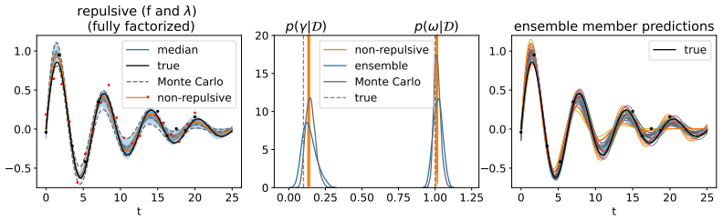
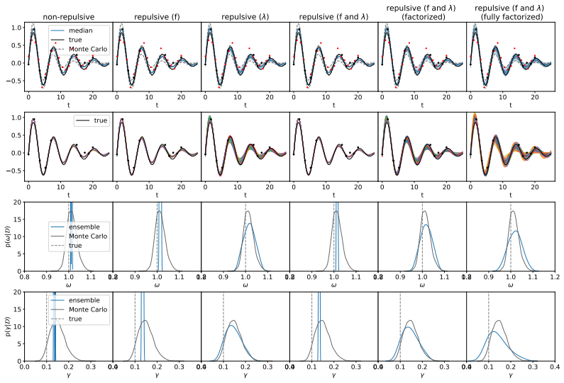
Recompute the exponential-equation reference posterior by Hamiltonian Monte Carlo using the prior the ensemble actually implements in function space—the prior on the initial condition and parameter mapped through the ODE solution with the correct Jacobian—and measure the Wasserstein distance between the fully-factorized repulsive ensemble and this reference as the ensemble grows from 25 to 250 members. The paper's claim predicts this distance shrinks toward zero; if it plateaus at a nonzero value once the prior mismatch is corrected, the ensemble is not converging to the true posterior. A cheaper check is latent in the paper's own Figure 3, where the joint-repulsion model's $W(\lambda)$ improves only slowly with ensemble size, so one can test whether the ensemble's marginal posterior for $\lambda$ approaches the MCMC marginal at all as $N_e$ grows.
Extended reading notes
Core claim
The paper's central claim is that the repulsive-ensemble construction carries over to physics-informed neural networks essentially unchanged, provided repulsion acts on the joint space of function values and differential-equation parameters. Following the Wasserstein-gradient-flow derivation of repulsive ensembles, each member's loss becomes a data-fit term plus a physics-residual term, minus the log-prior $\log p(f_i, \lambda_i)$ plus the log-density $\log \rho(f_i, \lambda_i)$ of the ensemble's own current predictions, so each member is pulled toward high posterior density while being pushed away from the others. The ensemble density $\rho$ is estimated by kernel density estimation, which becomes exact with infinitely many members, so the steady state of the ensemble is the true posterior $p(f, \lambda | D)$. The experiments confirm the corollaries: a standard ensemble collapses to a maximum-a-posteriori estimate with grossly overconfident intervals, while the repulsive variants agree with Hamiltonian Monte Carlo baselines on the exponential equation and the damped harmonic oscillator, with the fully-factorized repulsion giving the most consistently good uncertainty estimates across all test problems.
Load-bearing premise
The claim of convergence to the true Bayesian posterior assumes the prior term in the loss is a genuine density on the function values that appear in the data fit, but the experiments instead place the prior on initial conditions and parameters at a single point and never correct for the change of variables, so the posterior the ensemble targets is not exactly the one the Monte Carlo baseline samples.
Editorial extensions
If this is right
- Plain ensembles of PINNs are not reliable uncertainty estimators: they collapse to MAP solutions and report intervals orders of magnitude too narrow, so any risk assessment built on them would be overconfident.
- Where MCMC is feasible, repulsive ensembles reproduce its posterior, offering an alternative that works directly in function space and needs no low-dimensional reformulation of the problem.
- Because every ensemble member is itself an approximate solution of the differential equation, the uncertainty intervals stay anchored to the space of admissible solutions, even across gaps in the data.
- Theoretically repulsion should act on the joint space $(f, \lambda)$, but in practice factorizing the ensemble density gives the best results, with the fully-factorized variant winning on test-set log-likelihood in nearly every experiment.
Reading between the lines
- The strongest residual gap between the ensemble and the MCMC posterior is traceable to the prior being placed on initial conditions and parameters without the change-of-variables Jacobian; correcting the loss by that Jacobian is a testable modification that would either close the gap or shift it elsewhere.
- The consistent success of the fully-factorized repulsion suggests that for PINN uncertainty, per-point marginal calibration matters more than joint calibration; one could test this by checking whether pointwise interval coverage matches nominal levels even though the joint distribution is over-dispersed.
- If the convergence claim holds as stated, the approach offers a path to Bayesian inference for inverse problems where MCMC mixes slowly, since cost scales with the number of ensemble members rather than chain length; the paper does not demonstrate this scaling advantage, but it is an immediate consequence of the method.
Editorial analysis
A structured set of objections, weighed in public.
Referee Report
Summary. The paper proposes RE-PINN, a repulsive-ensemble method for Bayesian uncertainty quantification in physics-informed neural networks. Building on D'Angelo and Fortuin (2021), the authors derive a loss function (Eq. 10) that adds a KDE-based repulsive term in the joint space of function values and differential-equation parameters, with the claim that the ensemble distribution converges to the true Bayesian posterior as the number of ensemble members grows. The method is evaluated on the exponential ODE, the damped harmonic oscillator, the advection PDE, and the Lotka-Volterra system, comparing non-repulsive, partially repulsive, factorized, and fully factorized variants against Hamiltonian Monte Carlo baselines where available. The empirical results show that repulsive ensembles give substantially better uncertainty calibration than standard ensembles.
Significance. If the central claim is correct, the method would offer a practical alternative to MCMC for Bayesian inference in PINNs, combining the scalability of deep ensembles with a principled posterior interpretation. The paper is transparent in its presentation: it provides code, compares against HMC/NUTS baselines, includes several ablations of the repulsive term, and reports both point accuracy and uncertainty metrics. The theoretical novelty is limited, since the derivation is a direct substitution of a joint state vector into an existing framework, but the empirical study is useful. The main weakness is that the experiments do not implement the same prior that appears in the theoretical loss, which undermines the 'true posterior' claim and the direct comparison to the MCMC baselines.
major comments (3)
- [Section 4, Eq. (10); Appendix C] The loss in Eq. (10) requires p(f, λ) to be a density on the joint space of function values f at the data points and the DE parameters λ. However, Appendix C defines priors on initial conditions and parameters, e.g., p(f0) ~ U(−10,10) and p(λ) ~ U(−10,10) for the exponential equation, and states that 'the same priors can be used by plugging them into (10)', meaning the prior is evaluated at f_i(0) and λ_i. The map from (f0, λ) to the function values f is deterministic only if the ODE is solved exactly; with the soft PINN loss, f is not confined to that manifold. Even in a hard-constraint limit, a change of variables from (f0, λ) to f would require a Jacobian determinant, which is not accounted for. Consequently, the effective prior in the experiments is not the density p(f, λ) used in the derivation of Eq. (10), so the ensemble targets a different posterior than the MCMC baseline. This affects the central 'true Bayesian posterior' claim in the abstract and the comparisons in Tables 3–5 and Figures 2–4. The authors should either define a proper prior on function values, or restate the claim to describe the posterior actually targeted by the implemented loss.
- [Appendix D.1] The PDE-loss weight f_λ in Eq. (10) is derived as f_λ = σ_f^2 N_c/(σ_F^2 N_d) from the assumed noise levels, but in the experiments it is set by hand and annealed during training, e.g., for the exponential equation it is 'chosen as 5 and then increased to 10 and 25 at iterations 7500 and 9000'. This means that the loss being minimized changes over time and does not correspond to a fixed Bayesian posterior with a single σ_F. The theoretical guarantee that the repulsive loss drives the ensemble to the posterior of a fixed model therefore does not directly apply to the training procedure used in the experiments. The authors should either report the implied σ_F for each experiment or justify annealing as an approximation that does not alter the claimed stationary distribution.
- [Appendix A.1, Eq. (19)] Equation (19) is mathematically incorrect: the Fokker-Planck equation in Eq. (18) is ∂ρ/∂t = ∇·(ρ ∇(log ρ − log π)), not −∇(log ρ − log π). The second equality as written is missing the factor ρ and the divergence. Since this appendix is the derivation of the repulsive update that underlies the method, the inconsistency should be corrected or the appendix should explicitly refer to the original derivation in D'Angelo and Fortuin (2021).
minor comments (4)
- [Appendix D.7, Figure 11 caption] The caption refers to 'Lotka-V olterra equations (12)', but the equations are numbered (25) in the appendix; the cross-reference should be corrected.
- [Section 5.1, text after Eq. (12)] The phrase 'The factor f0 is obtained automatically when evaluating f(0)' is unclear, since f0 is the value of the solution at t=0; it would be clearer to say that no separate parameter f0 is introduced because it is the network output at t=0.
- [Table 1] The caption says 'Green ticks indicate methods that constitute integral parts of the method described in the paper. Grey ticks indicate methods that were considered for comparison.' It is not immediately clear why this distinction is needed in an overview of related work, and the wording could be simplified.
- [Appendix B, Eq. (22)] The notation for the kernel density estimate writes '1/√(|h| N_e)' but h is a vector of bandwidths; the expression is ambiguous about whether the square root applies to the product of bandwidths. Clarifying the normalization would improve reproducibility.
Circularity Check
No significant circularity: the repulsive-term construction is imported from independent prior theory and validated against MCMC baselines, so the central claim does not reduce to its inputs.
full rationale
The paper's central claim is that loss (10) makes the ensemble distribution converge to the Bayesian posterior. That guarantee comes from D'Angelo and Fortuin (2021), an external, independently derived Wasserstein-gradient-flow result, which the paper adapts by substituting [f, λ] for f (Eqs. 5-8). No parameter is fitted to the MCMC posterior: the KDE bandwidths use a standard median heuristic, and the weighting factors fλ, fρ are fixed from noise levels, not tuned to the target. Validation compares against HMC/NUTS baselines with stated priors and against PDEBench data, so the agreement in Figures 2-4 is an external check that could have failed. The Appendix C statement that the same priors can be plugged into (10) is a potential prior-space mismatch (the loss calls for a density on f, λ, while the experiments specify a density on f0, λ without a Jacobian), but this is a correctness/calibration concern about target matching, not a circularity: the ensemble and baseline are not forced to agree by construction and the method's uncertainty estimates are not derived from the baseline values. Hence no step in the derivation chain is equivalent to its own input.
Assumptions & free parameters
free parameters (2)
- f_λ (PDE residual weight) =
5,10,25 (exponential); 1,5,10 (oscillator); 0.1 (advection); 0.5,1,2 (Lotka-Volterra)
- 1/sqrt(N_d) normalization for fully-factorized repulsion =
1/sqrt(N_d)
assumptions (5)
- standard math Wasserstein gradient flow converges to the target posterior in the limit of infinite particles
- standard math Kernel density estimation becomes exact as the number of ensemble members tends to infinity
- domain assumption The function-space updates can be projected onto network weights via the Jacobian and implemented as a loss
- ad hoc to paper The prior on (f, λ) is a valid density on function values at the data points
- domain assumption The MCMC posterior computed from exact ODE solutions is a proxy for the PINN posterior
Cite this review
Pith. "Pith review of Repulsive Ensembles for Bayesian Inference in Physics-informed Neural Networks." pith.science (2026). https://pith.science/paper/TBARESWI
@misc{pith2026250517308,
  author       = {Pith},
  title        = {Pith review of: Repulsive Ensembles for Bayesian Inference in Physics-informed Neural Networks},
  year         = {2026},
  howpublished = {\url{https://pith.science/paper/TBARESWI}},
  note         = {Machine review of arXiv:2505.17308}
}
read the original abstract
Physics-informed neural networks (PINNs) have proven an effective tool for solving differential equations, in particular when considering non-standard or ill-posed settings. When inferring solutions and parameters of the differential equation from data, uncertainty estimates are preferable to point estimates, as they give an idea about the accuracy of the solution. In this work, we consider the inverse problem and employ repulsive ensembles of PINNs (RE-PINN) for obtaining such estimates. The repulsion is implemented by adding a particular repulsive term to the loss function, which has the property that the ensemble predictions correspond to the true Bayesian posterior in the limit of infinite ensemble members. Where possible, we compare the ensemble predictions to Monte Carlo baselines. Whereas the standard ensemble tends to collapse to maximum-a-posteriori solutions, the repulsive ensemble produces significantly more accurate uncertainty estimates and exhibits higher sample diversity.
Figures


Figures from the paper (8 more)




Reference graph
Works this paper leans on
-
[1]
Physics-informed neural networks: A deep learning framework for solving forward and inverse problems involving nonlinear partial differential equations
Maziar Raissi, Paris Perdikaris, and George E Karniadakis. Physics-informed neural networks: A deep learning framework for solving forward and inverse problems involving nonlinear partial differential equations. Journal of Computational physics, 378: 0 686--707, 2019
2019
-
[2]
Scientific machine learning through physics--informed neural networks: W here we are and what’s next
Salvatore Cuomo, Vincenzo Schiano Di Cola, Fabio Giampaolo, Gianluigi Rozza, Maziar Raissi, and Francesco Piccialli. Scientific machine learning through physics--informed neural networks: W here we are and what’s next. Journal of Scientific Computing, 92 0 (3): 0 88, 2022
work page 2022
-
[3]
Physics-informed neural networks ( PINN s) for fluid mechanics: A review
Shengze Cai, Zhiping Mao, Zhicheng Wang, Minglang Yin, and George Em Karniadakis. Physics-informed neural networks ( PINN s) for fluid mechanics: A review. Acta Mechanica Sinica, 37 0 (12): 0 1727--1738, 2021 a
work page 2021
-
[4]
Zaharaddeen Karami Lawal, Hayati Yassin, Daphne Teck Ching Lai, and Azam Che Idris. Physics-informed neural network ( PINN ) evolution and beyond: A systematic literature review and bibliometric analysis. Big Data and Cognitive Computing, 6 0 (4): 0 140, 2022
work page 2022
-
[5]
Physics-informed neural networks for heat transfer problems
Shengze Cai, Zhicheng Wang, Sifan Wang, Paris Perdikaris, and George Em Karniadakis. Physics-informed neural networks for heat transfer problems. Journal of Heat Transfer, 143 0 (6): 0 060801, 2021 b
work page 2021
-
[6]
Bayesian inference in statistical analysis
George EP Box and George C Tiao. Bayesian inference in statistical analysis. John Wiley & Sons, 2011
2011
-
[7]
Bayesian learning for neural networks, volume 118
Radford M Neal. Bayesian learning for neural networks, volume 118. Springer Science & Business Media, 2012
2012
-
[8]
Hands-on B ayesian neural networks-- A tutorial for deep learning users
Laurent Valentin Jospin, Hamid Laga, Farid Boussaid, Wray Buntine, and Mohammed Bennamoun. Hands-on B ayesian neural networks-- A tutorial for deep learning users. IEEE Computational Intelligence Magazine, 17 0 (2): 0 29--48, 2022
work page 2022
Show all 34 references
-
[9]
B- PINN s: B ayesian physics-informed neural networks for forward and inverse PDE problems with noisy data
Liu Yang, Xuhui Meng, and George Em Karniadakis. B- PINN s: B ayesian physics-informed neural networks for forward and inverse PDE problems with noisy data. Journal of Computational Physics, 425: 0 109913, 2021
2021
-
[10]
MCMC using H amiltonian dynamics
Radford M Neal et al. MCMC using H amiltonian dynamics. Handbook of markov chain monte carlo, 2 0 (11): 0 2, 2011
2011
-
[11]
Practical variational inference for neural networks
Alex Graves. Practical variational inference for neural networks. Advances in neural information processing systems, 24, 2011
2011
-
[12]
Dropout as a B ayesian approximation: R epresenting model uncertainty in deep learning
Yarin Gal and Zoubin Ghahramani. Dropout as a B ayesian approximation: R epresenting model uncertainty in deep learning. In international conference on machine learning, pages 1050--1059. PMLR, 2016
2016
-
[13]
Simple and scalable predictive uncertainty estimation using deep ensembles
Balaji Lakshminarayanan, Alexander Pritzel, and Charles Blundell. Simple and scalable predictive uncertainty estimation using deep ensembles. Advances in neural information processing systems, 30, 2017
2017
-
[14]
Stein variational gradient descent: A general purpose B ayesian inference algorithm
Qiang Liu and Dilin Wang. Stein variational gradient descent: A general purpose B ayesian inference algorithm. Advances in neural information processing systems, 29, 2016
2016
-
[15]
On linear identifiability of learned representations
Geoffrey Roeder, Luke Metz, and Durk Kingma. On linear identifiability of learned representations. In International Conference on Machine Learning, pages 9030--9039. PMLR, 2021
2021
-
[16]
F unction S pace P article O ptimization for B ayesian N eural N etworks
Ziyu Wang, Tongzheng Ren, Jun Zhu, and Bo Zhang. F unction S pace P article O ptimization for B ayesian N eural N etworks. In International Conference on Learning Representations, 2019
2019
-
[17]
Repulsive deep ensembles are B ayesian
Francesco D'Angelo and Vincent Fortuin. Repulsive deep ensembles are B ayesian. Advances in Neural Information Processing Systems, 34: 0 3451--3465, 2021
2021
-
[18]
The variational formulation of the F okker-- P lanck equation
Richard Jordan, David Kinderlehrer, and Felix Otto. The variational formulation of the F okker-- P lanck equation. SIAM journal on mathematical analysis, 29 0 (1): 0 1--17, 1998
1998
-
[19]
B ayesian neural network and B ayesian physics-informed neural network via variational inference for seismic petrophysical inversion
Peng Li, Dario Grana, and Mingliang Liu. B ayesian neural network and B ayesian physics-informed neural network via variational inference for seismic petrophysical inversion. Geophysics, 89 0 (6): 0 1--46, 2024
2024
-
[20]
Practical uncertainty quantification for space-dependent inverse heat conduction problem via ensemble physics-informed neural networks
Xinchao Jiang, Xin Wang, Ziming Wen, Enying Li, and Hu Wang. Practical uncertainty quantification for space-dependent inverse heat conduction problem via ensemble physics-informed neural networks. International Communications in Heat and Mass Transfer, 147: 0 106940, 2023
2023
-
[21]
Physics-informed neural networks for cardiac activation mapping
Francisco Sahli Costabal, Yibo Yang, Paris Perdikaris, Daniel E Hurtado, and Ellen Kuhl. Physics-informed neural networks for cardiac activation mapping. Frontiers in Physics, 8: 0 42, 2020
2020
-
[22]
Improved training of physics-informed neural networks with model ensembles
Katsiaryna Haitsiukevich and Alexander Ilin. Improved training of physics-informed neural networks with model ensembles. In 2023 International Joint Conference on Neural Networks (IJCNN), pages 1--8. IEEE, 2023
2023
-
[23]
Learning and discovering multiple solutions using physics-informed neural networks with random initialization and deep ensemble
Zongren Zou, Zhicheng Wang, and George Em Karniadakis. Learning and discovering multiple solutions using physics-informed neural networks with random initialization and deep ensemble. arXiv preprint arXiv:2503.06320, 2025
2025 arXiv
-
[24]
Ensemble learning for physics informed neural networks: A gradient boosting approach
Zhiwei Fang, Sifan Wang, and Paris Perdikaris. Ensemble learning for physics informed neural networks: A gradient boosting approach. arXiv preprint arXiv:2302.13143, 2023
2023 arXiv
-
[25]
Multi-output physics-informed neural networks for forward and inverse PDE problems with uncertainties
Mingyuan Yang and John T Foster. Multi-output physics-informed neural networks for forward and inverse PDE problems with uncertainties. Computer Methods in Applied Mechanics and Engineering, 402: 0 115041, 2022
2022
-
[26]
Evidential physics-informed neural networks
Hai Siong Tan, Kuancheng Wang, and Rafe McBeth. Evidential physics-informed neural networks. arXiv preprint arXiv:2501.15908, 2025
2025 arXiv
-
[27]
o ver, Bj \
Lennart R \"o ver, Bj \"o rn Malte Sch \"a fer, and Tilman Plehn. PINN ferring the H ubble function with uncertainties. energy, 5: 0 9, 2024
2024
-
[28]
Gradient flows: in metric spaces and in the space of probability measures
Luigi Ambrosio, Nicola Gigli, and Giuseppe Savar \'e . Gradient flows: in metric spaces and in the space of probability measures. Springer Science & Business Media, 2008
2008
-
[29]
Pdebench: A n extensive benchmark for scientific machine learning
Makoto Takamoto, Timothy Praditia, Raphael Leiteritz, Daniel MacKinlay, Francesco Alesiani, Dirk Pfl \"u ger, and Mathias Niepert. Pdebench: A n extensive benchmark for scientific machine learning. Advances in Neural Information Processing Systems, 35: 0 1596--1611, 2022
2022
-
[30]
Physics-informed neural networks with unknown measurement noise
Philipp Pilar and Niklas Wahlstr \"o m. Physics-informed neural networks with unknown measurement noise. In 6th Annual Learning for Dynamics & Control Conference, pages 235--247. PMLR, 2024
2024
-
[31]
Input-gradient space particle inference for neural network ensembles
Trung Trinh, Markus Heinonen, Luigi Acerbi, and Samuel Kaski. Input-gradient space particle inference for neural network ensembles. In The Twelfth International Conference on Learning Representations, 2024
2024
-
[32]
Chen, Martin Jankowiak, Fritz Obermeyer, Neeraj Pradhan, Theofanis Karaletsos, Rohit Singh, Paul Szerlip, Paul Horsfall, and Noah D
Eli Bingham, Jonathan P. Chen, Martin Jankowiak, Fritz Obermeyer, Neeraj Pradhan, Theofanis Karaletsos, Rohit Singh, Paul Szerlip, Paul Horsfall, and Noah D. Goodman. Pyro: Deep Universal Probabilistic Programming . Journal of Machine Learning Research, 2018
2018
-
[33]
The No-U-Turn sampler: adaptively setting path lengths in H amiltonian M onte C arlo
Matthew D Hoffman, Andrew Gelman, et al. The No-U-Turn sampler: adaptively setting path lengths in H amiltonian M onte C arlo. J. Mach. Learn. Res., 15 0 (1): 0 1593--1623, 2014
2014
-
[34]
Adam: A method for stochastic optimization
Diederik P Kingma and Jimmy Ba. Adam: A method for stochastic optimization. arXiv preprint arXiv:1412.6980, 2014
2014 arXiv
Reviewed August 7, 2026 · model on record in the stance chip above.
Discussion (0). Continue with ORCID to comment.