REVIEW 3 major objections 6 minor 33 references
Bayesian Deep Learning for Discrete Choice
T0 review · 3 major / 6 minor · reviewed 2026-08-07 · deepseek-v4-flash
Pith's one-line read A deep learning architecture for discrete choice that keeps 95% credible intervals honest while matching predictive baselines and producing behaviorally plausible value-of-travel-time estimates.
desk verdict Useful architecture and promising coverage results, but the posterior is not properly defined — fixed vs sampled scale parameters needs clarification before the Bayesian claims hold. read the letter →
The pith
A machine-rendered reading of the paper's core claim, the machinery that carries it, and where it could break.
The reading
What carries the argument
The load-bearing object is the representative-utility specification $v_{ij} = \alpha_j + x_{ij}^\top\beta + q_{ij}^\top\gamma + \sigma_{\mathrm{IIA}}\,\mathrm{BatchNorm}[f_{\Theta_f}(x_{ij}, q_{ij})] + \sigma_{\mathrm{nonIIA}}\,\mathrm{BatchNorm}[g_{\Theta_g}(x_i, q_i)_j]$, where the BatchNorm layers are non-affine (no learnable shift or scale) and $\sigma_{\mathrm{IIA}}$, $\sigma_{\mathrm{nonIIA}}$ are scale hyperparameters penalized by $\ell^2$ terms. These scales control how much the nonlinear components can contribute relative to the linear knowledge-informed part, so the model collapses to a standard linear discrete choice model when the data do not support nonlinear structure. The two-step training procedure first optimizes the log-posterior with the nonlinear layers frozen, then unfreezes them and runs SGLD to sample from the posterior; this steers the sampler toward modes where simple behavioral hypotheses have high posterior mass.
What would settle it
Run the Monte Carlo study with a different SGLD step-size schedule or chain length and compute trace-based convergence diagnostics; if empirical coverage of the marginal-rate-of-substitution intervals drops materially, the reported 94-99% coverage is an artifact of the specific sampler settings. A sharper version: on one simulated dataset, replace SGLD with a well-mixing Hamiltonian Monte Carlo sampler and compare the resulting credible intervals for the four MRS values; if the intervals differ substantially, the SGLD chain is not sampling the intended posterior.
Extended reading notes
Core claim
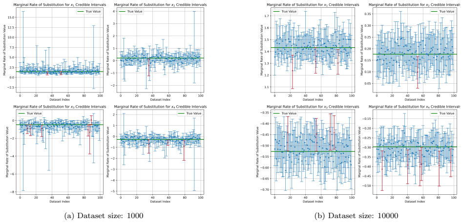
The authors claim that a deep learning discrete choice model can be made safe for economic inference by designing the architecture around a knowledge-informed component and by controlling the nonlinear blocks with non-affine batch normalization and scale hyperparameters. With their two-step procedure, fit the linear part with nonlinearities frozen and then run SGLD, the posterior credible intervals for marginal rates of substitution achieve empirical coverage of 94-99% in a 100-dataset Monte Carlo study at both N=1000 and N=10000 (Table 3), versus 79-84% for a fully connected neural network at N=1000 and 24-54% for a conditional logit model on the nonlinear MRS. The same setup produces value-of-travel-time estimates that are positive and behaviorally plausible in NYC and Swiss train data, with out-of-sample accuracy competitive with or better than baselines.
Load-bearing premise
The coverage results rest on the assumption that SGLD, after the two-step warm-start and with non-affine BatchNorm and fixed scale parameters, actually draws samples from the intended posterior over all model parameters; the paper supplies no convergence diagnostics, step-size schedule, or proof of this, and if the sampler targets a different distribution, the claimed 95% credible intervals are not supported.
Editorial extensions
If this is right
- Credible intervals for economic quantities such as marginal rates of substitution and value of travel time can be obtained from a deep learning model by pushing SGLD posterior samples through the marginal-utility function.
- The model's empirical coverage stays near the nominal 95% level at both N=1000 and N=10000, while a fully connected neural network undercovers at N=1000 and a conditional logit model misses the nonlinear MRS values.
- The posterior credible bands for latent utilities narrow as data grow, which the authors read as evidence that their SGLD implementation captures epistemic uncertainty.
- The model matches or beats baselines on out-of-sample accuracy, improving by 8 percentage points in simulations as N grows and outperforming the state-of-the-art benchmark by 6 percentage points on the Swiss route choice data.
- Stronger $\ell^2$ penalties on the nonlinear scale parameters push the model toward the linear, behaviorally informed specification, and the model produces positive value-of-travel-time estimates even with no penalty.
Reading between the lines
- Editorial inference: a testable extension is to monitor the posterior mass on $\sigma_{\mathrm{IIA}}$ and $\sigma_{\mathrm{nonIIA}}$; if the collapse-to-linear mechanism works, these scales should shrink toward zero when data are scarce and grow when nonlinear structure is present.
- Editorial inference: the two-step warm-start is doing substantial work, so an SGLD run from a random initialization might explore behaviorally implausible modes; a counterfactual study with random initialization would isolate how much of the coverage and VOTT behavior comes from the initialization rather than the sampler.
- Editorial inference: the architecture's scaling mechanism is generic and could be combined with other approximate inference methods such as SWAG, deep ensembles, or variational inference, and with other economic quantities such as elasticities and willingness-to-pay distributions, provided the same two-step stabilization is used.
- Editorial inference: because no convergence diagnostics are reported, the coverage numbers are the only evidence that the sampler is targeting the intended posterior; applying standard MCMC diagnostics would either strengthen or qualify the central claim.
Editorial analysis
A structured set of objections, weighed in public.
Referee Report
Summary. The paper proposes a deep learning architecture for discrete choice that combines a knowledge-informed linear utility component, an IIA nonlinear block, and a non-IIA nonlinear block, with scale parameters sigma_IIA and sigma_nonIIA controlling the contribution of the nonlinearities. Training uses a two-step procedure: first optimize the log-posterior with the nonlinear layers frozen, then run Stochastic Gradient Langevin Dynamics after unfreezing. The authors evaluate the method in a Monte Carlo study with simulated data, reporting empirical coverage of credible intervals for marginal rates of substitution (Table 3: 94-99% for their model at N=1000 and N=10000), and present two case studies in which their model yields behaviorally plausible values of travel time savings. The central claim is that this architecture, combined with SGLD, provides valid approximate Bayesian inference for economic quantities while retaining competitive predictive accuracy.
Significance. If the central claim holds, the paper addresses a genuine gap: deep learning models for discrete choice have so far offered point predictions but not a demonstrated route to interval estimation for quantities like marginal rates of substitution. The architecture's built-in collapse to a linear, behaviorally informed model when nonlinearities are unsupported is a useful inductive bias, and the simulation study against a fully connected neural network and a conditional logit model is informative. The empirical coverage results in Table 3 are a strong piece of evidence, and the case studies illustrate that the method can produce economically plausible estimates in real applications. However, the significance is currently conditional on resolving a load-bearing ambiguity in the definition of the posterior and on providing evidence that the SGLD sampler actually targets that posterior.
major comments (3)
- [Section 5, Eqs. (11) and (14)] The target posterior is not defined consistently. Equation (11) explicitly interprets the L2 penalties on sigma_IIA and sigma_nonIIA as Gaussian priors, which makes these scale parameters random quantities, while Equation (14) defines theta as (beta, Theta_f, Theta_g), excludes sigma_IIA and sigma_nonIIA, and states that they 'are fixed because they are treated as hyperparameters during learning.' If the sigmas are fixed at estimates from the first step, then the objective in Eq. (11) is a penalized likelihood conditional on those estimates, not a negative log-posterior over the sampled parameters, and the intervals in Eqs. (17)-(19) are conditional on point estimates of sigma, ignoring their uncertainty. If the sigmas are instead sampled, then Eqs. (14)-(15) omit part of the parameter vector and the pushforward is computed from the wrong posterior. The paper must specify which case holds and adjust the Bayesian interpretation and coverage claims accordingly, otherwise Table 3 cannot be read as evidence of Bayesian credible intervals.
- [Section 5.2 and Table 3] The paper provides no convergence diagnostics or implementation details for the SGLD sampler, and this is load-bearing because the coverage results in Table 3 are the main evidence for the method. The only information given is 'SGLD with 5,000 epochs'; there is no step-size schedule, no burn-in or thinning description, no number of retained samples, and no trace plots or other diagnostics demonstrating that the iterates approximate draws from p(theta|D). In addition, the architecture uses batch-normalization layers with batch statistics, and it is not explained how the batch-dependent normalization affects either the gradient in the SGLD update of Eq. (8) or the derivative computation m_ijk(theta) in Eq. (14). The authors should report the exact SGLD configuration, provide diagnostics or sensitivity checks, and clarify whether batch or running statistics are used when evaluating m_ijk, or the coverage numbers cannot be attributed to correct posterior sampling.
- [Sections 6 and 8.1] The simulation study is underreported to the point of not being reproducible. The data-generating parameters beta, gamma, and Phi are not given; the statement that Phi was selected to give 'around 70% weighted out-of-sample accuracy' is not a substitute for reporting the parameter values. The authors also do not define precisely how the 'average marginal rate of substitution' intervals are constructed: for each simulated dataset, is the average taken over individuals within each posterior draw before computing quantiles, or are individual-level posterior means averaged? The SGLD hyperparameters needed to reproduce Table 3 (step-size schedule, batch size, burn-in, thinning, number of retained samples) are absent. These details should be added so that the empirical coverage results can be independently verified.
minor comments (6)
- [Eq. (13)] The marginal rate of substitution is conventionally defined with a negative sign (dx_k/dx_l = - (du/dx_l)/(du/dx_k)); the sign convention used here should be stated explicitly, especially since the case studies report positive values of travel time savings.
- [Abstract and Tables 4-6] The abstract mentions 'out-of-sample balanced accuracy,' but the results report 'weighted out-of-sample accuracy'; these terms should be reconciled and the metric defined precisely.
- [Tables 5 and 6] The 'SOTA' rows in Tables 5 and 6 are not tied to a specific reference in the text; the footnote markers appear to be missing, so the reader cannot tell which published model the comparison is against.
- [Section 5.1] The statement that the two-step procedure 'ensures' the model defaults to the behaviorally informed hypothesis is stronger than what is demonstrated; it would be more accurate to say that the procedure is designed to do so and that the simulations support this behavior.
- [Eq. (6)] The notation in Eq. (6) conditions on y on both sides of the equation, which appears to be a typo; the predictive density should condition on the observed training data and covariates only.
- [Figures 14-17] The VOTT histograms are posterior-mean summaries and are presented without credible intervals; adding interval summaries would make the inference in the case studies more complete and better aligned with the paper's emphasis on uncertainty quantification.
Circularity Check
No significant circularity: coverage is validated against external simulated ground truth, and the self-citations are contextual, not load-bearing.
full rationale
The paper's central quantitative claim, the 94-99% empirical coverage in Table 3, is not circular. The true marginal rates of substitution are computed from the known data-generating process ('we compare them with the true marginal rates of substitution, computed using the known function parameters and their derivatives', Sec. 6), and the SGLD credible intervals are produced by the architecture and sampling procedure described in Secs. 5 and 8, not derived from the coverage numbers. No fitted parameter is renamed as a prediction: sigma_IIA and sigma_nonIIA are scales with L2 penalties, and their values are not used to define the target MRS in the simulation. The self-citations ([10], [31]) provide prior architecture and behavioral reference ranges, but they do not carry the derivation of the coverage or VOTT results, which are implemented and evaluated in this paper. There is a statistical coherence concern that sigma_IIA and sigma_nonIIA are described as having Gaussian priors in Eq. (11) but are fixed as hyperparameters in Sec. 5.2, so the sampled posterior may not match the stated posterior; however, that is a misspecification/correctness issue, not a circular reduction of output to input. I found no self-definitional prediction, no fitted input relabeled as prediction, and no load-bearing self-citation chain.
Assumptions & free parameters
free parameters (4)
- Simulation nonlinearity parameters Phi =
not reported (hand-selected for ~70% accuracy)
- SGLD step size schedule and number of retained samples =
not reported
- Regularization hyperparameters lambda_IIA, lambda_nonIIA =
cross-validated in case studies; fixed at 0.0001 in simulation (footnote 5)
- Network architecture hyperparameters (layers, hidden units) =
512 hidden units, 2 layers in simulation; cross-validated in case studies
assumptions (3)
- standard math SGLD converges to the posterior p(theta | D) under the stated step-size and noise conditions (Welling and Teh 2011).
- ad hoc to paper The two-step warm-start and subsequent SGLD sampling target the same posterior p(theta | D).
- ad hoc to paper BatchNorm layers with batch statistics do not compromise posterior sampling or the derivative computation m_ijk(theta).
Cite this review
Pith. "Pith review of Bayesian Deep Learning for Discrete Choice." pith.science (2026). https://pith.science/paper/53N76C5N
@misc{pith2026250518077,
  author       = {Pith},
  title        = {Pith review of: Bayesian Deep Learning for Discrete Choice},
  year         = {2026},
  howpublished = {\url{https://pith.science/paper/53N76C5N}},
  note         = {Machine review of arXiv:2505.18077}
}
read the original abstract
Discrete choice models (DCMs) are used to analyze individual decision-making in contexts such as transportation choices, political elections, and consumer preferences. DCMs play a central role in applied econometrics by enabling inference on key economic variables, such as marginal rates of substitution, rather than focusing solely on predicting choices on new unlabeled data. However, while traditional DCMs offer high interpretability and support for point and interval estimation of economic quantities, these models often underperform in predictive tasks compared to deep learning (DL) models. Despite their predictive advantages, DL models remain largely underutilized in discrete choice due to concerns about their lack of interpretability, unstable parameter estimates, and the absence of established methods for uncertainty quantification. Here, we introduce a deep learning model architecture specifically designed to integrate with approximate Bayesian inference methods, such as Stochastic Gradient Langevin Dynamics (SGLD). Our proposed model collapses to behaviorally informed hypotheses when data is limited, mitigating overfitting and instability in underspecified settings while retaining the flexibility to capture complex nonlinear relationships when sufficient data is available. We demonstrate our approach using SGLD through a Monte Carlo simulation study, evaluating both predictive metrics--such as out-of-sample balanced accuracy--and inferential metrics--such as empirical coverage for marginal rates of substitution interval estimates. Additionally, we present results from two empirical case studies: one using revealed mode choice data in NYC, and the other based on the widely used Swiss train choice stated preference data.
Figures


Figures from the paper (12 more)




Reference graph
Works this paper leans on
-
[1]
S. Wang, B. Mo, S. Hess, J. Zhao, Comparing hundreds of machine learning classifiers and discrete choice models in predicting travel behavior: an empirical benchmark, arXiv preprint arXiv:2102.01130 (2021)
arXiv 2021
-
[2]
S. Wang, Q. Wang, J. Zhao, Deep neural networks for choice analysis: Extracting complete economic information for interpretation, Transportation Research Part C: Emerging Technologies 118 (2020) 102701
work page 2020
-
[3]
A. G. Wilson, P. Izmailov, Bayesian deep learning and a probabilistic perspective of generalization, Advances in neural information processing systems 33 (2020) 4697–4708
2020
-
[4]
A. G. Wilson, The case for bayesian deep learning, arXiv preprint arXiv:2001.10995 (2020)
arXiv 2020
-
[5]
Y. Han, F. C. Pereira, M. Ben-Akiva, C. Zegras, A neural-embedded discrete choice model: Learning taste representation with strengthened interpretability, Transportation Research Part B: Methodological 163 (2022) 166–186
work page 2022
-
[6]
J. Lu, Y. Meng, H. Timmermans, A. Zhang, Modeling hesitancy in airport choice: A comparison of discrete choice and machine learning methods, Transportation Research Part A: Policy and Practice 147 (2021) 230–250
work page 2021
-
[7]
S. Wang, B. Mo, J. Zhao, Deep neural networks for choice analysis: Architecture design with alternative-specific utility functions, Transportation Research Part C: Emerging Technologies 112 (2020) 234–251
work page 2020
-
[8]
S. Feng, R. Yao, S. Hess, R. A. Daziano, T. Brathwaite, J. Walker, S. Wang, Deep neural networks for choice analysis: Enhancing behavioral regularity with gradient reg- ularization, Transportation Research Part C: Emerging Technologies 166 (2024) 104767
work page 2024
Show all 33 references
-
[9]
B.Sifringer, V.Lurkin, A.Alahi, Enhancingdiscretechoicemodelswithneuralnetworks, in: 18th Swiss Transport Research Conference, 2018, pp. 1–3
2018
-
[10]
D. F. Villarraga, R. A. Daziano, Designing graph convolutional neural networks for discrete choice with network effects, arXiv preprint arXiv:2503.09786 (2025)
2025 arXiv
-
[11]
A. N. Angelopoulos, S. Bates, A gentle introduction to conformal prediction and distribution-free uncertainty quantification, arXiv preprint arXiv:2107.07511 (2021)
2021 arXiv
-
[12]
A. N. Angelopoulos, R. F. Barber, S. Bates, Theoretical foundations of conformal prediction, arXiv preprint arXiv:2411.11824 (2024). 35
2024 arXiv
-
[13]
Papamarkou, M
T. Papamarkou, M. Skoularidou, K. Palla, L. Aitchison, J. Arbel, D. Dunson, M. Filippone, V. Fortuin, P. Hennig, J. M. Hernandez-Lobato, et al., Position: Bayesian deep learning is needed in the age of large-scale ai, arXiv preprint arXiv:2402.00809 (2024). URL:[https://arxiv....
2024 arXiv
-
[14]
W. J. Maddox, P. Izmailov, T. Garipov, D. P. Vetrov, A. G. Wilson, A simple baseline for bayesian uncertainty in deep learning, Advances in neural information processing systems 32 (2019)
2019
-
[15]
Welling, Y
M. Welling, Y. W. Teh, Bayesian learning via stochastic gradient langevin dynamics, in: Proceedings of the 28th international conference on machine learning (ICML-11), Citeseer, 2011, pp. 681–688
2011
-
[16]
K. E. Train, Discrete Choice Methods with Simulation, 2 ed., Cambridge University Press, 2009. doi:10.1017/CBO9780511805271
2009 doi
-
[17]
Zheng, Z
S. Zheng, Z. Fang, L. Zhao, Incorporating uncertainty quantification into travel mode choice modeling: a bayesian neural network (bnn) approach and an uncertainty-guided active survey framework, arXiv preprint arXiv:2406.10948 (2024)
2024 arXiv
-
[18]
Arkoudi, R
I. Arkoudi, R. Krueger, C. L. Azevedo, F. C. Pereira, Combining discrete choice mod- els and neural networks through embeddings: Formulation, interpretability and perfor- mance, Transportation research part B: methodological 175 (2023) 102783
2023
-
[19]
M. Wong, B. Farooq, Reslogit: A residual neural network logit model for data-driven choice modelling, Transportation Research Part C: Emerging Technologies 126 (2021) 103050
2021
-
[20]
A. G. Wilson, P. Izmailov, Bayesian deep learning and a probabilistic perspective of generalization, arXiv (2020).arXiv:2002.08791
2020 arXiv
-
[21]
H. Li, Z. Xu, G. Taylor, C. Studer, T. Goldstein, Visualizing the loss landscape of neural nets, Advances in Neural Information Processing Systems 2018-December (2018) 6389–6399.arXiv:1712.09913
2018 arXiv
-
[22]
A. E. Raftery, D. Madigan, J. A. Hoeting, Bayesian Model Averaging for Linear Re- gression Models, Journal of the American Statistical Association 92 (1997) 179–191. doi:10.1080/01621459.1997.10473615
1997
-
[23]
Izmailov, D
P. Izmailov, D. Podoprikhin, T. Garipov, D. Vetrov, A. G. Wilson, Averaging weights leads to wider optima and better generalization, arXiv preprint arXiv:1803.05407 (2018)
2018 arXiv
-
[24]
H. Li, Z. Xu, G. Taylor, C. Studer, T. Goldstein, Visualizing the loss landscape of neural nets, Advances in neural information processing systems 31 (2018). 36
2018
-
[25]
Lakshminarayanan, A
B. Lakshminarayanan, A. Pritzel, C. Blundell, Simple and scalable predictive uncer- tainty estimation using deep ensembles, Advances in Neural Information Processing Systems 2017-December (2017) 6403–6414.arXiv:1612.01474
2017 arXiv
-
[26]
D. J. C. MacKay, Bayesian interpolation, Neural Computation 4 (1992) 415–447. URL:[https://doi.org/10.1162/neco.1992.4.3.415](https: //doi.org/10.1162/neco.1992.4.3.415). doi:10.1162/neco.1992.4.3.415. arXiv:[https://direct.mit.edu/neco/article-pdf/4/3/415/812340/neco.1992.4.3...
1992 doi
-
[27]
S. Wang, B. Mo, J. Zhao, Theory-based residual neural networks: A synergy of discrete choice models and deep neural networks, Transportation research part B: methodological 146 (2021) 333–358
2021
-
[28]
Ioffe, C
S. Ioffe, C. Szegedy, Batch normalization: Accelerating deep network training by re- ducing internal covariate shift, in: International conference on machine learning, pmlr, 2015, pp. 448–456
2015
-
[29]
J. Yi, M. A. Bessa, Cooperative bayesian and variance networks disentangle aleatoric and epistemic uncertainties, arXiv preprint arXiv:2505.02743 (2025)
2025 arXiv
-
[30]
Sarrias, R
M. Sarrias, R. A. Daziano, Individual-specific point and interval conditional estimates of latent class logit parameters, Journal of choice modelling 27 (2018) 50–61
2018
-
[31]
D. F. Villarraga, R. A. Daziano, Hierarchical nearest neighbor gaus- sian process models for discrete choice: Mode choice in new york city, Transportation Research Part B: Methodological 191 (2025) 103132. URL: [https://www.sciencedirect.com/science/article/pii/S01912615240025...
2025
-
[32]
Vrtic, K
M. Vrtic, K. W. Axhausen, The impact of tilting trains in switzerland: A route choice model of regional-and long distance public transport trips, Arbeitsberichte Verkehrs-und Raumplanung 128 (2002)
2002
-
[33]
Q. Li, X. Yuan, J. Xie, Combination of gnn and mnl: a new model for deal- ing with multi-classification tasks, Applied Mathematics and Nonlinear Sciences 9 (2024). URL:[https://doi.org/10.2478/amns-2024-3548](https://doi.org/10. 2478/amns-2024-3548). doi:10.2478/amns-2024-3548. 37
2024 doi
Reviewed August 7, 2026 · model on record in the stance chip above.
Discussion (0). Sign in to comment.