REVIEW 4 major objections 7 minor 50 references
Load Forecasting in the Era of Smart Grids: Opportunities and Advanced Machine Learning Models
T0 review · 4 major / 7 minor · reviewed 2026-08-15 · deepseek-v4-flash
Pith's one-line read Machine-learning models beat the ARIMA baseline on a seven-day Arizona load forecast, with LSTM most accurate at 1.74% MAPE.
desk verdict A clearly written but methodologically under-powered benchmark; the ML-beats-ARIMA claim is plausible but confounded by an unfair baseline and a fragile evaluation protocol. read the letter →
The pith
A machine-rendered reading of the paper's core claim, the machinery that carries it, and where it could break.
The reading
What carries the argument
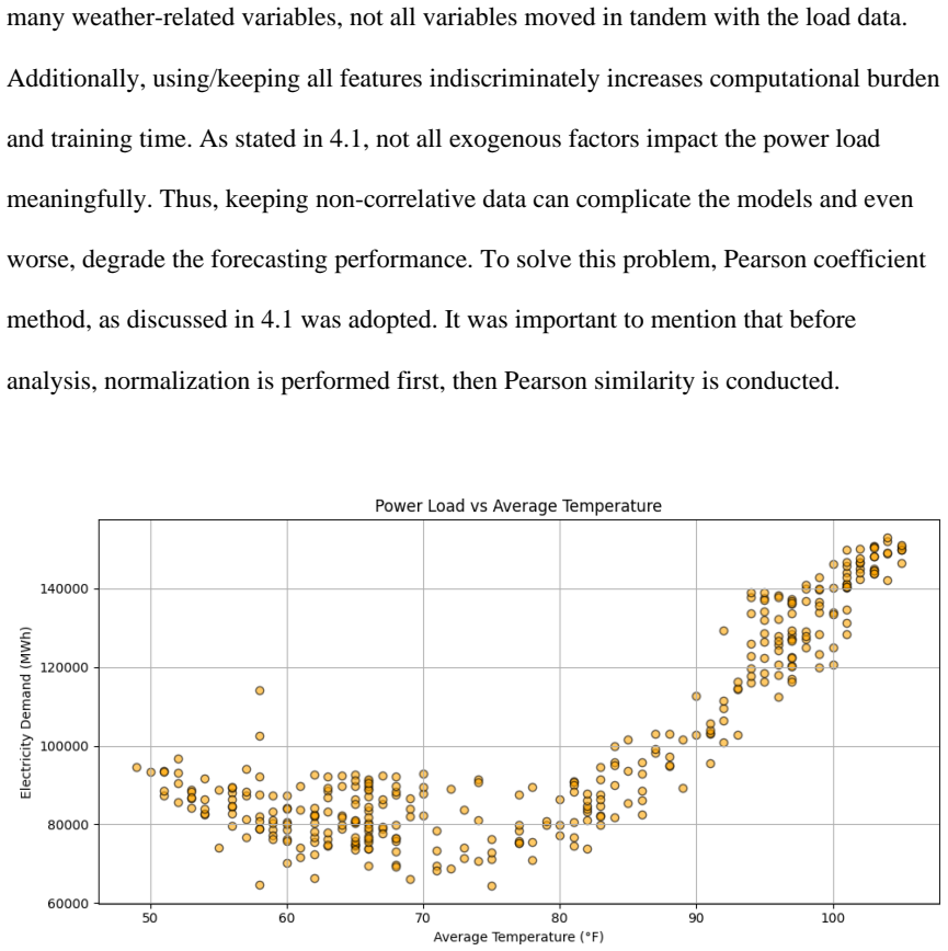
The argument is carried by a forecasting pipeline built on Pearson correlation feature selection, engineered time-series features, and a fixed train/test split. Pearson correlation coefficients pick exogenous weather variables that move with load—minimum temperature (0.86), maximum temperature (0.84), UV index (0.72)—and discard weak ones like wind speed and pressure. The models share features such as one-day lagged load, three- and seven-day rolling averages, and day-of-week indicators. The ARIMA baseline is selected via autocorrelation and partial autocorrelation plots after first-order differencing. The hybrid ARIMA-SVM model first fits ARIMA on the load series, then trains a support-vector regression on the residuals. The LSTM and GRU use gated recurrent units with stacked layers, dropout, and early stopping, while XGBoost and LightGBM are tuned with a custom random-search hyperparameter optimizer. The test protocol is a single seven-day holdout at the end of the dataset.
What would settle it
Rerun all six models on multiple rolling test windows, for example every month across a full year, and report per-window MAPE with error bars; if ARIMA wins on most windows or the ML ranking reverses, the central claim that machine learning improves forecasting on this dataset is unsupported.
Extended reading notes
Core claim
The paper's central discovery is that, on daily load data from an Arizona utility spanning 2020–2025, machine-learning models outperform the classical ARIMA baseline in short-term forecasting accuracy. Table 7.1 summarizes the ranking: LSTM has the lowest error (MAE 1535.71 MWh, MAPE 1.74%), followed by LightGBM (1708.22 MWh, 1.95%), hybrid ARIMA-SVM (1857.14 MWh, 2.09%), XGBoost (2039.53 MWh, 2.33%), and GRU (2178.57 MWh, 2.53%), all below ARIMA (3878.2 MWh, 4.03%). The author also finds that a naive XGBoost without custom hyperparameter tuning performs worse than ARIMA (MAPE 4.67%), and that LightGBM offers near-LSTM accuracy at lower computational cost.
Load-bearing premise
The evaluation assumes that the final seven days of the dataset are representative of out-of-sample conditions, so the reported error rankings and percentages could change if a different test period were used.
Editorial extensions
If this is right
- For daily ahead load forecasts, using LSTM or LightGBM instead of ARIMA can roughly halve mean absolute percentage error.
- The hybrid ARIMA-SVM result shows that modeling the nonlinear residual after a linear baseline is a viable route to improved accuracy.
- Hyperparameter tuning is decisive for tree-based models: untuned XGBoost underperforms ARIMA, while tuned XGBoost beats it by a wide margin.
- LSTM is the most accurate but computationally heavier, so LightGBM is a credible cost-effective alternative.
- For an arid climate, temperature-based features dominate load variation, so future models can focus on temperature and calendar features.
Reading between the lines
- Beyond the paper's claims, a single seven-day test window is unlikely to pin down the ranking among the top models; multiple rolling test windows could change the ordering.
- Daily aggregation hides intraday peaks that matter for unit commitment, so the same models applied to hourly data might show different relative strengths.
- The strong temperature-load correlation in Arizona suggests the models' advantage may depend on climate; a transfer test on a humid or cold region would clarify how general the finding is.
- The author's own caveat that past data cannot fully represent future or present events points toward incremental retraining and real-time weather pipelines as a natural next test.
Signed reviews
Editorial analysis
A structured set of objections, weighed in public.
Referee Report
Summary. The manuscript, an arXiv posting of an Arizona State University Master's thesis, reports a short-term daily load forecasting study for the APS balancing authority using EIA load data and NOAA weather data. It implements a univariate ARIMA baseline, a hybrid ARIMA-SVM model, XGBoost, LightGBM, LSTM, and GRU, with Pearson-correlation-based feature selection and MAE/MAPE evaluation on a final 7-day holdout. The central claim is that, for this dataset, all machine-learning models beat the ARIMA baseline, with LSTM best at MAPE 1.74%. The writing is clear and the implementation descriptions are detailed, but the empirical comparison is confounded, and the current evidence does not support the claimed ranking or the magnitude of the ML advantage.
Significance. If the comparison were clean, the result would be a modest, directionally consistent confirmation that nonlinear models with exogenous features can improve daily load forecasts over a plain univariate ARIMA. The manuscript is transparent about the ARIMA baseline's lack of exogenous inputs (Section 5.1) and about test-set-based tuning of LightGBM (Section 5.3.2), which is a credit to the authors but does not remove the problems. It does not provide a matched-input classical competitor, a multi-window evaluation, uncertainty quantification, or code/data availability, so the significance of the quantitative claims is currently limited.
major comments (4)
- [§5.1, §5.4.1, Table 7.1] The headline ML-versus-ARIMA comparison is confounded by input features. Section 5.1 states that the ARIMA baseline 'only relies on past load values and does not consider exogenous factors such as weather data, holidays, or other calendar events,' whereas the XGBoost, LightGBM, LSTM, and GRU models are given temperature and calendar features (Tables 5.2, 5.4, and Sections 5.3 and 5.4.1). The large error gap in Table 7.1 may therefore reflect additional information rather than machine learning per se. A classical or statistical model given the same exogenous inputs, such as ARIMAX or a linear regression with temperature, day-of-week, and holiday indicators, must be added before the abstract's claim can be supported; as written, the comparison does not isolate the contribution of the ML machinery.
- [§5.3.2, Table 6.4] LightGBM hyperparameters were selected by optimizing MAPE on the test set, as stated in Section 5.3.2: the optimizer identified configurations 'that produced the most accurate forecasts on the test set.' This makes the reported LightGBM result (and therefore its rank in Table 7.1) optimistic relative to a genuine out-of-sample evaluation. The selection must be moved to a validation split or done with time-series cross-validation as was done for XGBoost in Section 5.3.1, and the final test-set results should be reported only after selection is frozen.
- [§5.3.1, §6.3–6.8] All model metrics are computed on a single final 7-day test window, with no repeated holdout periods, error bars, or significance tests. Sections 6.3 through 6.8 each report one MAE/MAPE pair for one week, and Section 5.3.1 states that 'the final 7 days of the dataset were held out as the test set.' With only seven daily observations, the ranking among LSTM, LightGBM, and the hybrid model could easily change under a different test period. A rolling-origin or multi-window backtest with mean and spread of metrics, and ideally a Diebold-Mariano test on the daily errors, is needed to support any ranking claim.
- [§4.2.3, §4.4] The manuscript does not state whether normalization and Pearson-correlation feature selection are computed on the training split only. Section 4.4 says 'before analysis, normalization is performed first, then Pearson similarity is conducted,' but not whether the min-max statistics and the correlations include the test period. If the full 2020–2025 sample is used for preprocessing, test information leaks into all models, and the reported generalization errors are too optimistic. The authors should either clarify that all preprocessing statistics were estimated on the training portion or re-run the pipeline with split-only statistics.
minor comments (7)
- [Eq. (4.10)] The MAPE formula in Eq. (4.10) is missing absolute values; it should be MAPE = (100/n) Σ |A_t − F_t| / A_t.
- [Eq. (4.13), Section 4.3] 'RSME' is a typo for RMSE in Eq. (4.13) and in the surrounding text.
- [Appendix A] The acronym list defines GRU as 'Gradient Recurring Unit'; the correct expansion is 'Gated Recurrent Unit,' as used in Sections 5.4.2 and 6.8.
- [Section 7] The chapter numbering skips from Section 7.1 to 7.3; there is no Section 7.2, which creates a structural gap.
- [Section 6.5] The text says 'Figure 6.2 shows the output of the XGBoost model' but the referenced figure is Figure 6.3; please correct the cross-reference.
- [Section 6.6] The unoptimized LightGBM result (MAPE 2.18%, MAE 1984.5) is mentioned only in prose and not included in Table 6.4; adding it would make the tuning comparison reproducible.
- [References] References [45] and [46] appear to be the same paper (Khalil et al., 'Economic LSTM Approach'); the duplicate should be removed and the citation list renumbered.
Circularity Check
LightGBM's reported forecast error is a test-set-tuned quantity, but the broader ML-over-ARIMA claim has independent support.
-
fitted input called prediction
[Section 5.3.2 (LightGBM tuning), with results reported in Section 6.6 (Table 6.4) and Section 7.1 (Table 7.1)]
"Rather than relying solely on manual tuning, or default researched values, this approach involved programmatically testing multiple combinations of hyperparameters to identify those that produced the most accurate forecasts on the test set."
The same final 7-day evaluation window used for all reported metrics is used here as the selection objective: LightGBM hyperparameters are chosen by minimizing MAPE on the test set, and Table 6.4/7.1 then reports that same test-set MAPE (1.95%) as the model's forecast performance. The reported value is therefore not an independent out-of-sample prediction for LightGBM; it is the minimum over the tried configurations on the evaluation window, so the apparent improvement from 2.18% to 1.95% is partly a selection artifact. This does not make the whole ML-vs-ARIMA conclusion circular, because untuned LightGBM, XGBoost, LSTM, GRU, and the hybrid also beat the ARIMA baseline; it mainly makes LightGBM's precise error and its rank in Table 7.1 forced by construction.
full rationale
No derivation chain or equations in the thesis reduce to their own inputs; this is an empirical comparison, not a mathematical derivation, and there is no load-bearing self-citation. The one demonstrated circular step is the LightGBM hyperparameter selection on the test set, whose reported MAPE is the very objective used for selection. The rest of the evaluation is substantially independent: XGBoost hyperparameters are chosen by three-fold time-series cross-validation on the training portion (Section 5.3.1), LSTM/GRU use early stopping on training loss, and the hybrid ARIMA-SVM follows the standard residual-decomposition approach. The central claim that ML models beat a classical ARIMA baseline is also supported by models whose results were not test-set-tuned. Two evaluation weaknesses are noted but are not circularity: the ARIMA baseline receives no weather/calendar inputs while ML models do, so part of the error gap could reflect information advantage rather than algorithm class; and the single 7-day test window with no significance tests leaves the exact ranking unstable. The thesis also does not state whether normalization and Pearson feature selection were computed on the training split only (Sections 4.2.3 and 4.4); if full-data statistics were used, feature selection would ingest test-period information, but the text does not exhibit this explicitly, so it is not scored as a circular step.
Assumptions & free parameters
free parameters (6)
- XGBoost hyperparameters =
n_estimators=300, max_depth=5, learning_rate=0.06, subsample=0.8, colsample_bytree=0.8, random_state=42
- LightGBM hyperparameters =
n_estimators=300, max_depth=5, learning_rate=0.06, subsample=0.4, colsample_bytree=1.0, random_state=50
- LSTM architecture hyperparameters =
2 LSTM layers of 50 units, dropouts 0.3/0.2, Adam lr=0.005, MAE loss, 14-day windows, early stopping
- GRU architecture hyperparameters =
2 GRU layers of 100 and 50 units, dropouts 0.3/0.2, Adam lr=0.005, 3-day lags
- Preprocessing thresholds alpha(t), beta(t), delta(t) =
not specified
- Holdout window length =
7 days
assumptions (4)
- domain assumption Historical load and weather patterns remain representative for the forecast horizon
- domain assumption Pearson correlation is a sufficient basis for feature selection
- domain assumption EIA and NOAA data are accurate and aligned
- domain assumption Normalization and correlation statistics do not use test-period information
Cite this review
Pith. "Pith review of Load Forecasting in the Era of Smart Grids: Opportunities and Advanced Machine Learning Models." pith.science (2026). https://pith.science/paper/PMHSKU5F
@misc{pith2026250518170,
  author       = {Pith},
  title        = {Pith review of: Load Forecasting in the Era of Smart Grids: Opportunities and Advanced Machine Learning Models},
  year         = {2026},
  howpublished = {\url{https://pith.science/paper/PMHSKU5F}},
  note         = {Machine review of arXiv:2505.18170}
}
read the original abstract
Electric energy is difficult to store, requiring stricter control over its generation, transmission, and distribution. A persistent challenge in power systems is maintaining real-time equilibrium between electricity demand and supply. Oversupply contributes to resource wastage, while undersupply can strain the grid, increase operational costs, and potentially impact service reliability. To maintain grid stability, load forecasting is needed. Accurate load forecasting balances generation and demand by striving to predict future electricity consumption. This thesis examines and evaluates four machine learning frameworks for short term load forecasting, including gradient boosting decision tree methods such as Extreme Gradient Boosting (XGBoost) and Light Gradient Boosting Machine (LightGBM). A hybrid framework is also developed. In addition, two recurrent neural network architectures, Long Short Term Memory (LSTM) networks and Gated Recurrent Units (GRU), are designed and implemented. Pearson Correlation Coefficient is applied to assess the relationships between electricity demand and exogenous variables. The experimental results show that, for the specific dataset and forecasting task in this study, machine learning-based models achieved improved forecasting performance compared to a classical ARIMA baseline.
Figures


Figures from the paper (26 more)






Reference graph
Works this paper leans on
-
[1]
U.S. DOE, “FOTW #1365, October 21, 2024: U.S. Net Generation of Electricity Relied on Record Use of Renewables while Coal Use Dropped to a Record Low in 2023,” Office of Energy Efficiency & Renewable Energy, Oct. 21, 2024
work page 2024
-
[2]
Intelligent Systems for Power Load Forecasting: a Study Review,
I. S. Jahan, V. Snasel, and S. Misak, “Intelligent Systems for Power Load Forecasting: a Study Review,” Energies, vol. 13, no. 22, p. 6105, Nov. 2020, doi: https://doi.org/10.3390/en13226105
-
[3]
Deep Learning Modeling in Electricity Load forecasting: Improved Accuracy by Combining DWT and LSTM,
Seyed Azad Nabavi, S. Mohammadi, Naser Hossein Motlagh, Sasu Tarkoma, and P. Geyer, “Deep Learning Modeling in Electricity Load forecasting: Improved Accuracy by Combining DWT and LSTM,” Energy Reports, vol. 12, no. 2, pp. 2873–2900, Dec. 2024, doi: https://doi.org/10.1016/j.egyr.2024.08.070
-
[4]
J. Zheng, C. Xu, Z. Zhang, and X. Li, “Electric Load Forecasting in Smart Grids Using Long-Short-Term-Memory Based Recurrent Neural Network,” 2017 51st Annual Conference on Information Sciences and Systems (CISS), vol. i, no. 1, Mar. 2017, doi: https://doi.org/10.1109/ciss.2017.7926112
arXiv 2017
-
[5]
A General Framework for Load Forecasting Based on Pre-trained Large Language Model,
M. Gao, S. Zhou, W. Gu, Z. Wu, H. Liu, and A. Zhou, “A General Framework for Load Forecasting Based on Pre-trained Large Language Model,” Arxiv.org, 2018. https://arxiv.org/html/2406.11336v2
arXiv 2018
-
[6]
Accurate Electricity Load Forecasting with Artificial Neural Networks,
D. Ortiz-Arroyo, M. K. Skov, and Q. Huynh, “Accurate Electricity Load Forecasting with Artificial Neural Networks,” Computational Intelligence for Modelling, Control and Automation, 2005. pp. 94–99, Dec. 2005, doi: https://doi.org/10.1109/CIMCA.2005.1631248
-
[7]
Machine Learning Basics and Potential Applications in Power Systems,
T. Xue, U. Karaagac, I. Kocar, M. B. Vavdareh, and M. Ghafouri, “Machine Learning Basics and Potential Applications in Power Systems,” 2023 International Conference on Electrical, Communication and Computer Engineering (ICECCE), pp. 1–7, Dec. 2023, doi: https://doi.org/10.1109/icecce61019.2023.10441935
arXiv 2023
-
[8]
P. Kaledio, “Machine Learning Applications in Electric Power Systems: Enhancing Efficiency, Reliability, and Sustainability,” SSRN Electronic Journal, Jan. 2024, doi: https://doi.org/10.2139/ssrn.4716389
Show all 50 references
-
[9]
Load Forecasting in Applied Mathematics for Power Systems,
E. A. Feinberg and D. Genethliou, “Load Forecasting in Applied Mathematics for Power Systems,” Power Electronics and Power Systems, pp. 269–285, Aug. 2019, doi: https://doi.org/10.1007/0-387-23471-3_12. 71
2019 doi
-
[10]
Long-term Load forecasting: Models Based on MARS, ANN and LR Methods,
G. Nalcaci, A. Özmen, and G. W. Weber, “Long-term Load forecasting: Models Based on MARS, ANN and LR Methods,” Central European Journal of Operations Research, vol. 27, no. 4, pp. 1033–1049, Mar. 2018, doi: https://doi.org/10.1007/s10100-018-0531-1
2018 doi
-
[11]
Methods and Models for Electric Load Forecasting: A Comprehensive Review,
M. A. Hammad, B. Jereb, B. Rosi, and D. Dragan, “Methods and Models for Electric Load Forecasting: A Comprehensive Review,” Logistics & Sustainable Transport, vol. 11, no. 1, pp. 51–76, Feb. 2020, doi: https://doi.org/10.2478/jlst- 2020-0004
2020 doi
-
[12]
Load Forecasting Techniques for Power System: Research Challenges and Survey,
N. Ahmad, Y. Ghadi, M. Adnan, and M. Ali, “Load Forecasting Techniques for Power System: Research Challenges and Survey,” IEEE Xplore, pp. 1–15, Jul. 2022, doi: https://doi.org/10.1109/access.2022.3187839
2022
-
[13]
Short-term Electricity Load forecasting—A Systematic Approach from System Level to Secondary Substations,
M. G. Pinheiro, S. C. Madeira, and A. P. Francisco, “Short-term Electricity Load forecasting—A Systematic Approach from System Level to Secondary Substations,” Applied Energy, vol. 332, pp. 120493–120493, Feb. 2023, doi: https://doi.org/10.1016/j.apenergy.2022.120493
2023
-
[14]
Long Term Load Forecasting with Hourly Predictions Based on long-short-term-memory Networks,
R. K. Agrawal, F. Muchahary, and M. M. Tripathi, “Long Term Load Forecasting with Hourly Predictions Based on long-short-term-memory Networks,” IEEE Xplore, Feb. 18, 2018. https://ieeexplore.ieee.org/stamp/stamp.jsp?tp=&arnumber=8312088
2018
-
[15]
Short-Term Load Forecasting Method Based on ARIMA and LSTM,
S. Chen, R. Lin, and W. Zeng, “Short-Term Load Forecasting Method Based on ARIMA and LSTM,” 2022 IEEE 22nd International Conference on Communication Technology (ICCT), pp. 1913–1917, Mar. 2023, doi: https://doi.org/10.1109/icct56141.2022.10073051
2022
-
[16]
Forecasting: Principles and Practice,
R. J. Hyndman and G. Athanasopoulos, “Forecasting: Principles and Practice,” Otexts.com, 2018. https://otexts.com/fpp2/
2018
-
[17]
Time Series Analysis: Forecasting and Control,
G. E. P. Box and G. M. Jenkins, “Time Series Analysis: Forecasting and Control,” 1970
1970
-
[18]
A Comprehensive Review of the Load Forecasting Techniques Using Single and Hybrid Predictive Models,
A. Al Mamnun, MD. Sohel, N. Mohammad, S. Haque, and D. Roy Dipta, “A Comprehensive Review of the Load Forecasting Techniques Using Single and Hybrid Predictive Models,” Jun. 26, 2020. https://ieeexplore.ieee.org/stamp/stamp.jsp?arnumber=9144528
2020
-
[19]
Comparison of ARIMA and SVM for Short- term Load Forecasting,
M. A. A. Amin and Md. A. Hoque, “Comparison of ARIMA and SVM for Short- term Load Forecasting,” IEEE Xplore, Oct. 21, 2019. https://ieeexplore.ieee.org/stamp/stamp.jsp?tp=&arnumber=8877077. 72
2019
-
[20]
Short-Term Load Foresting Using Combination of Linear and Non-linear Models,
N. Rani, S. K. Aggarwal, and S. Kumar, “Short-Term Load Foresting Using Combination of Linear and Non-linear Models,” IEEE Access, vol. 1, no. 1, pp. 1–1, Apr. 2024, doi: https://doi.org/10.1109/access.2024.3392592
2024
-
[21]
SARIMA Modelling for Forecasting the Electricity Consumption of a Health Care Building,
H. Kaur and S. Ahuja, “SARIMA Modelling for Forecasting the Electricity Consumption of a Health Care Building,” International Journal of Innovative Technology and Exploring Engineering, vol. 8, no. 12, pp. 2795–2799, Oct. 2019, doi: https://doi.org/10.35940/ijitee.l2575.1081219
2019
-
[22]
ARIMA Models in Electrical Load Forecasting and Their Robustness to Noise,
E. Chodakowska, J. Nazarko, and Ł. Nazarko, “ARIMA Models in Electrical Load Forecasting and Their Robustness to Noise,” Energies, vol. 14, no. 23, p. 7952, Nov. 2021, doi: https://doi.org/10.3390/en14237952
2021 doi
-
[23]
Application of a Load Forecasting Model Based on Improved Grey Neural Network in the Smart Grid,
N. Tang and D.-J. Zhang, “Application of a Load Forecasting Model Based on Improved Grey Neural Network in the Smart Grid,” Energy Procedia, vol. 12, pp. 180–184, 2011, doi: https://doi.org/10.1016/j.egypro.2011.10.025
2011 doi
-
[24]
Short Term Load Forecasting Using Multiple Linear Regression,
N. Amral, C. S. Ozveren, and D. King, “Short Term Load Forecasting Using Multiple Linear Regression,” IEEE Xplore, Oct. 04, 2007. https://ieeexplore.ieee.org/document/4469121
2007
-
[25]
Short Term Load Forecasting Based on ARIMA and ANN Approaches,
C. Tarmanini, N. Sarma, C. Gezegin, and O. Ozgonenel, “Short Term Load Forecasting Based on ARIMA and ANN Approaches,” Energy Reports, vol. 9, no. 3, pp. 550–557, May 2023, doi: https://doi.org/10.1016/j.egyr.2023.01.060
2023 doi
-
[26]
Electrical load forecasting using support vector machines,
B. Emre Türkay and D. Demren, “Electrical load forecasting using support vector machines,” 7th International Conference on Electrical and Electronics Engineering (ELECO), vol. 1, no. 1, Dec. 2011, doi: https://ieeexplore.ieee.org/document/6140142
2011
-
[27]
Application of Support Vector Machine and Similar Day Method for Load Forecasting,
X. Li, C. Sun, and D. Gong, “Application of Support Vector Machine and Similar Day Method for Load Forecasting,” Springer Nature Link, vol. 1, no. 1, pp. 602– 609, 2005, doi: https://doi.org/10.1007/11539117_85
2005 doi
-
[28]
Neural Networks for short-term Load forecasting: A Review and Evaluation,
H. S. Hippert, C. E. Pedreira, and R. C. Souza, “Neural Networks for short-term Load forecasting: A Review and Evaluation,” IEEE Transactions on Power Systems, vol. 16, no. 1, pp. 44–55, 2001, doi: https://doi.org/10.1109/59.910780
2001 doi
-
[29]
Nature-inspired Algorithms for feed-forward Neural Network classifiers: a Survey of One Decade of Research,
A. M. Hemeida et al., “Nature-inspired Algorithms for feed-forward Neural Network classifiers: a Survey of One Decade of Research,” Ain Shams Engineering Journal, vol. 11, no. 3, pp. 659–675, Sep. 2020, doi: https://doi.org/10.1016/j.asej.2020.01.007. 73
2020 doi
-
[30]
Long-Term Power Load Forecasting Using LSTM-Informer with Ensemble Learning,
K. Wang, J. Zhang, X. Li, and Y. Zhang, “Long-Term Power Load Forecasting Using LSTM-Informer with Ensemble Learning,” Electronics, vol. 12, no. 10, p. 2175, May 2023, doi: https://doi.org/10.3390/electronics12102175
2023 doi
-
[31]
Load Forecasting Based on Smart Meter Data and Gradient Boosting Decision Tree,
X. Yu, Z. Xu, X. Zhou, J. Zheng, Y. Xia, and L. Lin, “Load Forecasting Based on Smart Meter Data and Gradient Boosting Decision Tree,” 2019 Chinese Automation Congress (CAC), vol. 1, no. 1, Feb. 2020, doi: https://doi.org/10.1109/cac48633.2019.8996810
2019
-
[32]
Prediction of Home Energy Consumption Based on Gradient Boosting Regression Tree,
P. Nie, M. Roccotelli, M. P. Fanti, Z. Ming, and Z. Li, “Prediction of Home Energy Consumption Based on Gradient Boosting Regression Tree,” Energy Reports, vol. 7, pp. 1246–1255, Nov. 2021, doi: https://doi.org/10.1016/j.egyr.2021.02.006
2021 doi
-
[33]
Energy Consumption Forecasts by Gradient Boosting Regression Trees,
L. Di Persio and N. Fraccarolo, “Energy Consumption Forecasts by Gradient Boosting Regression Trees,” Mathematics, vol. 11, no. 5, p. 1068, Feb. 2023, doi: https://doi.org/10.3390/math11051068
2023 doi
-
[34]
Short-Term Load Forecasts Using LSTM Networks,
S. Muzaffar and A. Afshari, “Short-Term Load Forecasts Using LSTM Networks,” Energy Procedia, vol. 158, pp. 2922–2927, Feb. 2019, doi: https://doi.org/10.1016/j.egypro.2019.01.952
2019 doi
-
[35]
Electrical Load Forecasting Using LSTM, GRU, and RNN Algorithms,
M. Abumohsen, A. Y. Owda, and M. Owda, “Electrical Load Forecasting Using LSTM, GRU, and RNN Algorithms,” Energies, vol. 16, no. 5, p. 2283, Feb. 2023, doi: https://doi.org/10.3390/en16052283
2023 doi
-
[36]
Daily Average Load Demand Forecasting Using LSTM Model Based on Historical Load Trends,
R. Bareth, A. Yadav, S. Gupta, and M. Pazoki, “Daily Average Load Demand Forecasting Using LSTM Model Based on Historical Load Trends,” IET Generation, Transmission & Distribution, vol. 18, no. 5, pp. 952–962, Feb. 2024, doi: https://doi.org/10.1049/gtd2.13132
2024 doi
-
[37]
Load Forecasting Based on LSTM Neural Network and Applicable to Loads of ‘Replacement of Coal with Electricity,’
Z. Chen et al., “Load Forecasting Based on LSTM Neural Network and Applicable to Loads of ‘Replacement of Coal with Electricity,’” Journal of Electrical Engineering & Technology, vol. 16, no. 5, pp. 2333–2342, Apr. 2021, doi: https://doi.org/10.1007/s42835-021-00768-8
2021 doi
-
[38]
Short-Term Residential Load Forecasting Based on LSTM Recurrent Neural Network,
W. Kong, Z. Y. Dong, Y. Jia, D. J. Hill, Y. Xu, and Y. Zhang, “Short-Term Residential Load Forecasting Based on LSTM Recurrent Neural Network,” IEEE Transactions on Smart Grid, vol. 10, no. 1, pp. 841–851, Oct. 2017, doi: https://doi.org/10.1109/tsg.2017.2753802
2017
-
[39]
Short-Term Load Forecasting Using an LSTM Neural Network,
M. M. Hossain and H. Mahmood, “Short-Term Load Forecasting Using an LSTM Neural Network,” 2020 IEEE Power and Energy Conference at Illinois (PECI), Feb. 2020, doi: https://doi.org/10.1109/peci48348.2020.9064654. 74
2020
-
[40]
Understanding LSTM Networks,
C. Olah, “Understanding LSTM Networks,” Colah’s Blog, Aug. 27, 2015. https://colah.github.io/posts/2015-08-Understanding-LSTMs/
2015
-
[41]
Heterogeneous Transfer Learning on Power Systems: A Merged Multi-modal Gaussian Graphical Model,
H. Li, Y. Weng, and H. Tong, “Heterogeneous Transfer Learning on Power Systems: A Merged Multi-modal Gaussian Graphical Model,” 2021 IEEE International Conference on Data Mining (ICDM), Nov. 2020, doi: https://doi.org/10.1109/icdm50108.2020.00130
2021
-
[42]
Incorporating Air Temperature into mid-term Electricity Load Forecasting Models Using time-series Regressions and Neural Networks,
N. Bashiri Behmiri, C. Fezzi, and F. Ravazzolo, “Incorporating Air Temperature into mid-term Electricity Load Forecasting Models Using time-series Regressions and Neural Networks,” Energy, vol. 278, p. 127831, Sep. 2023, doi: https://doi.org/10.1016/j.energy.2023.127831
2023
-
[43]
Effects of Various Factors on Electric Load forecasting: an Overview,
S. Khatoon, Ibraheem, A. K. Singh, and Priti, “Effects of Various Factors on Electric Load forecasting: an Overview,” 2014 6th IEEE Power India International Conference (PIICON), Jun. 2015, doi: https://doi.org/10.1109/poweri.2014.7117763
2014
-
[44]
Regularizing and Optimizing LSTM Language Models,
S. Merity, N. Shirish Keskar, and R. Socher, “Regularizing and Optimizing LSTM Language Models,” arXiv, vol. 1, no. 1, Aug. 2017, Available: https://arxiv.org/pdf/1708.02182
2017 arXiv
-
[46]
Economic LSTM Approach for Recurrent Neural Networks,
K. Khalil, O. Eldash, A. Kumar, and M. Bayoumi, “Economic LSTM Approach for Recurrent Neural Networks,” IEEE Transactions on Circuits & Systems II Express Briefs, vol. 66, no. 11, pp. 1885–1889, Jun. 2019, doi: https://doi.org/10.1109/tcsii.2019.2924663
2019
-
[47]
A Review of Machine Learning Applications in Power System Resilience,
J. Xie, Inalvis Alvarez-Fernandez, and W. Sun, “A Review of Machine Learning Applications in Power System Resilience,” IEEE Xplore, vol. 1, no. 1, Aug. 2020, doi: https://doi.org/10.1109/pesgm41954.2020.9282137
2020
-
[48]
Hybrid of ARIMA and SVMs for Short- Term Load Forecasting,
H. Nie, G. Liu, X. Liu, and Y. Wang, “Hybrid of ARIMA and SVMs for Short- Term Load Forecasting,” Energy Procedia, vol. 16, pp. 1455–1460, 2012, doi: https://doi.org/10.1016/j.egypro.2012.01.229
2012 doi
-
[49]
Hybrid Short Term Load Forecasting Using ARIMA-SVM,
S. Karthika, V. Margaret, and K. Balaraman, “Hybrid Short Term Load Forecasting Using ARIMA-SVM,” IEEE Xplore, Apr. 01, 2017. https://ieeexplore.ieee.org/document/8245060. 75
2017
-
[50]
Forecasting Electricity Load with Hybrid Scalable Model Based on Stacked Non Linear Residual Approach,
A. Sinha, R. Tayal, A. Vyas, P. Pandey, and O. P. Vyas, “Forecasting Electricity Load with Hybrid Scalable Model Based on Stacked Non Linear Residual Approach,” Frontiers in Energy Research, vol. 9, no. 1, Nov. 2021, doi: https://doi.org/10.3389/fenrg.2021.720406
2021
-
[51]
Hybrid Adaptive Techniques for electric- load Forecast Using ANN and ARIMA,
A. A. El Desouky and M. M. El Kateb, “Hybrid Adaptive Techniques for electric- load Forecast Using ANN and ARIMA,” IEE Proceedings - Generation, Transmission and Distribution, vol. 147, no. 4, p. 213, 2010, doi: https://doi.org/10.1049/ip-gtd:20000521. 76 APPENDIX A ACRONYMS A...
2010 doi
Reviewed August 15, 2026 · model on record in the stance chip above.
Discussion (0). Continue with ORCID to comment.