REVIEW 4 major objections 5 minor 58 references
Dynamically Polarized SERF Atomic Comagnetometer
T0 review · 4 major / 5 minor · reviewed 2026-08-07 · deepseek-v4-flash
Pith's one-line read A K-Rb-21Ne SERF comagnetometer can be run in a pulsed, dynamically polarized mode that suppresses pump-light polarization noise by 38.5% and low-frequency magnetic-field response by 51.1% when the duty ratio is raised from 40% to 60%…
desk verdict A useful experimental extension of pulsed-pumping SERF comagnetometry to a hybrid K-Rb-21Ne system, with credible direct measurements but headline suppression numbers that need error bars and a chirp check before I'd take them at face value. read the letter →
The pith
A machine-rendered reading of the paper's core claim, the machinery that carries it, and where it could break.
The reading
What carries the argument
The load-bearing object is the three-phase evolutionary model for the coupled alkali-noble-gas spin ensemble. In Phase I, nuclear spin polarization is described by exponential polarization and depolarization with a constant relaxation rate, giving a steady longitudinal nuclear polarization proportional to the duty ratio, $P_n^{{(I)}}$_z = D_r $P_n^{{(DC)}}$_z. Phase II is the pump-on steady state of the electron spins, obtained from the Bloch equations with the real pump rate; it supplies the compensation point and the initial conditions for free precession. Phase III is the pump-off damped oscillation, modeled after the electron polarization has decayed to near zero as a fixed-frequency linear process, fit with the formula $P_x^{{(III)}}$(t) = exp(-$R_2^{{(III)}}$ t / $Q^{{(III)}}$) [A_sin sin(2π f t + φ_Ω) + A_cos cos(2π f t + φ_Ω)] + B exp(-$R_1^{{(III)}}$ t / $Q^{{(III)}}$) + C. The amplitudes A_sin and A_cos are the readouts that separate the two transverse axes, and the assumption of slow frequency drift in the chosen 20-35 ms window is what makes the analytical fit possible.
What would settle it
Measure the instantaneous frequency of the Phase III damped signal across the 20-35 ms window using a short-time Fourier transform or Hilbert transform while holding the duty ratio fixed. If the instantaneous frequency changes by more than the frequency resolution within that window, the fixed-frequency linear assumption fails and the fitted A_sin and A_cos values are biased. A complementary check is to integrate the full Bloch equations with a density-matrix solver and compare the recovered amplitudes with the analytical fixed-frequency fit; disagreement indicates model bias.
Extended reading notes
Core claim
The paper's central claim is that a SERF comagnetometer can be driven by pulsed pump light rather than continuous pumping, and that the resulting dynamic polarization is analytically tractable and technically advantageous. In the K-Rb-21Ne setup, K electron spins are pumped along z and transfer polarization to Rb and then to 21Ne; once the pump is switched off at 11 Hz, the electron spins depolarize within tens of milliseconds while the nuclear polarization remains nearly fixed, leaving the electron spins to undergo damped free precession around the residual field. The authors divide this cycle into three phases and derive analytical solutions for each: nuclear polarization settles to a value proportional to the duty ratio (Phase I), electron spins reach a DC-like steady state while the pump is on (Phase II), and after pump-off the damped oscillation in a frequency-stable window (Phase III) is fit with a fixed-frequency sinusoid whose sine and cosine amplitudes separate the x- and y-axis responses. With this model they report an average 38.5% suppression of pump-light-induced polarization noise and an average 51.1% suppression of the low-frequency magnetic-field response when the duty ratio goes from 40% to 60%, and they show that the same compensation point works in both pump-on and pump-off phases.
Load-bearing premise
The Phase III fits assume that after the electron polarization has decayed to near zero, the precession frequency changes slowly enough over the 20-35 ms fitting window that the damped oscillation can be treated at fixed frequency; if the frequency drifts within that window, the fitted amplitudes A_sin and A_cos are biased in a way that would distort the reported suppression percentages.
Editorial extensions
If this is right
- Operating the comagnetometer in the pump-off phase reduces the response to pump-light intensity fluctuations: the reported average suppression is 38.5% relative to the pump-on steady state.
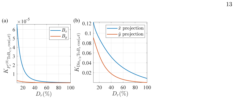
- Raising the duty ratio from 40% to 60% increases the nuclear longitudinal polarization in proportion to the duty ratio and suppresses the low-frequency magnetic-field response by an average 51.1%, so dynamic polarization preserves self-compensation.
- The fitted amplitudes A_sin and A_cos separate the responses to rotations about two orthogonal axes, enabling dual-axis inertial rotation measurement during free precession.
- In the low-frequency band below about 0.1 Hz the pulsed scheme improves sensitivity compared with the pump-on steady state; above 0.1 Hz sensitivity is limited by background noise and magnetic-field instability near the cell.
- Using the fitting parameters instead of a single time point of the damped signal reduces the noise floor by about 36.3%.
Reading between the lines
- The same three-phase split would likely transfer to other hybrid alkali-noble-gas sensors with widely separated electron and nuclear relaxation times, so the model may describe Rb-Xe comagnetometers and pulsed atomic clocks that measure free precession.
- Because raising the duty ratio suppresses low-frequency magnetic-field response but also lowers the rotation scale factor, an optimal duty ratio should exist for a given magnetic-field stability budget; the paper does not optimize this trade-off.
- The pump-off measurement window creates a natural stroboscopic geometry, so combining the scheme with squeezed or entangled probe light could in principle reach below the standard quantum limit, though the paper only mentions such extensions as future work.
- The reported 38.5% and 51.1% values are averages over the tested duty-ratio and frequency ranges; a direct extension would map these suppression percentages as functions of pump modulation frequency and duty ratio and compare them with the model's predictions at other operating points.
Signed reviews
Editorial analysis
A structured set of objections, weighed in public.
Referee Report
Summary. This manuscript reports a K-Rb-21Ne SERF comagnetometer operated with pulsed pump light at 11 Hz, with duty ratios varied from 40% to 60%. The authors propose a three-phase evolutionary model of the coupled electron-nuclear spin dynamics, present a magnetic-field compensation procedure based on the pump-on steady state, and characterize the response to inertial rotation, low-frequency magnetic fields, and pump-light intensity fluctuations during the pump-off phase. The headline quantitative results are an averaged 38.5% suppression of pump-light-induced polarization noise and an averaged 51.1% suppression of the low-frequency magnetic-field response when the duty ratio is increased from 40% to 60%.
Significance. If the quantitative claims are correct, the pulsed-pump scheme is a useful technical addition to SERF comagnetometry: it reduces sensitivity to pump-light fluctuations and low-frequency magnetic fields without abandoning self-compensation. The experimental work is substantial: the setup includes a K-Rb-21Ne cell, AOM-based pump modulation, and a full three-axis compensation procedure, and the responses are measured at five duty ratios. The paper's honesty about limiting factors (magnetic-field stability near the cell, electric heating, and the small Phase III scale factor) is commendable. The main weakness is that the central suppression percentages are extracted from fits to a linearized damped-oscillation model whose key assumption—slowly varying precession frequency—is asserted but not quantitatively validated. The 'complete analytical solution' is actually an approximate piecewise model with many fitted parameters, and the manuscript does not provide code or processed data tables, only data available upon request.
major comments (4)
- [II.D, Eq. (2), and II.E, Eq. (3)] The suppression percentages (38.5% and 51.1%) are derived from the fitted amplitudes A_sin and A_cos in Eq. (3), which assumes a strictly constant precession frequency f = gamma_e(B_z+B_n0)/Q^(III). The paper's own model makes Q^(III) time-dependent through the decaying longitudinal electron polarization, and the stated value Q^(III)=10.27 corresponds to P_e^z ~ 18%, which is not 'near zero.' The only justification for the linearization is the qualitative statement that the frequency 'changes slowly,' plus one RMSE value (4.01e-5 V) for a single fit. This is insufficient: a fit with a time-dependent phase (e.g., f(t)=f0+beta t) or fits in sliding sub-windows should be compared to Eq. (3) to bound the frequency drift over the 20–35 ms window. Because the decay trajectory at the start of Phase III depends on the duty ratio, any frequency-drift bias would enter A_sin and A_cos differentially across the five duty ratios and could shift the headline suppression values.
- [Abstract and METHODS, Eq. (8)] The claim of a 'complete analytical solution' for the spin dynamics is overstated. The three-phase model is a piecewise approximation: Phase I uses an equivalent mean pumping rate, Phase II uses the steady state, and Phase III explicitly 'can be approximated as a linear evolution process' (Methods). The resulting expressions contain many fitted parameters (Q, R_e1/Q, R_e2/Q, f, B_n0, A, B, C, phi, A_sin, A_cos, k_e) and are not closed-form in the usual sense. Recommend rephrasing to 'approximate analytical solution' and stating the validity conditions quantitatively.
- [II.F, Fig. 6] The 51.1% suppression figure is described only as an 'average' over the low-frequency magnetic field responses, but the averaging rule is not given. It is not specified how the ratio is computed across the tested frequency range (0.005–1 Hz), across the Bx and By axes, or across the five duty ratios, nor is an uncertainty or confidence interval provided. The figure shows outliers attributed to 'system drift' without quantitative criteria. Please provide a table of the per-frequency, per-axis, per-duty-ratio response coefficients used to compute the 51.1% average, and report the standard error of the mean.
- [II.G, Fig. 7] The 38.5% suppression of pump-light fluctuations is reported as an 'overall average of all collected data,' but only two duty ratios (50% and 55%) are shown, and no statistical uncertainty or number of measurements is given. The definition of the 'relative response coefficient' also needs clarification: it is the slope of light-intensity fluctuation against A_cos or P_e^(II)_x, divided by the scale factor with respect to Omega_y, but the units of the light-intensity fluctuation (photodiode voltage) and the normalization must be stated explicitly. Please report the per-frequency values and their errors.
minor comments (5)
- [Fig. 4(a)] Consider plotting the residuals of the fit; one RMSE value for a single representative trace does not convey the fit quality across duty ratios.
- [METHODS, Eqs. (6)-(8)] The notation {R_e2, R_e2, R_e1} is nonstandard; please define it as a diagonal matrix acting on the polarization vector.
- [Inset of Fig. 4] Report the fitted slope k and its uncertainty for the linear relation B_n0 versus duty ratio.
- [II.E] The differential measurement with points 180 degrees apart is described too briefly; specify how the two points are combined to remove bias.
- [II.H, Eq. (5)] Define all symbols in Eq. (5), including the units of S, K_Omega, and the noise terms.
Circularity Check
No significant circularity: the suppression percentages are direct measurements and the model is not used as its own confirmation.
full rationale
The central quantitative claims are empirical. The 51.1% low-frequency magnetic-field suppression (Sec. II.F, Fig. 6) is a ratio of measured response coefficients obtained from fitting the damped-oscillation waveform of Eq. 3 at duty ratios from 40% to 60%, and the 38.5% polarization-noise suppression (Sec. II.G, Fig. 7) is a comparison of measured relative response coefficients to pump-light modulation. Neither quantity is forced by the theoretical model. The three-phase model (Sec. II.A and Methods Eqs. 6-14) is an analytical solution of the Bloch equations under stated approximations; it predicts the association of A_sin/A_cos with rotation and magnetic-field inputs, but the experiment tests that association rather than defining it. Self-citations such as Refs. [37] and [43] are used as calibration and measurement-procedure references, not as a load-bearing uniqueness argument or as an alternative to independent data. The most plausible concern is the fixed-frequency Phase III approximation in Eqs. 2-3: if the precession frequency drifts appreciably within the 20-35 ms fitting window, the fitted A_sin and A_cos amplitudes could be biased, potentially shifting the reported suppression percentages. That is a model-misspecification and robustness risk, not a circular dependency between input and output; assessing it would require a comparison against a chirp or time-dependent-phase fit, not a circularity correction.
Assumptions & free parameters
free parameters (6)
- Q(III) slowing-down factor =
10.27 (average)
- Electron relaxation rates R_e2(III)/Q(III) and R_e1(III)/Q(III) =
not reported separately
- Precession frequency f =
values in Fig. 4
- Nuclear effective magnetic field B_n0 =
linear fit vs duty ratio (inset Fig. 4)
- Damped-oscillation amplitudes, offset, and phase (A, B, C, phi, A_sin, A_cos) =
not reported
- Decay coefficient k_e =
not reported
assumptions (5)
- domain assumption The spin-exchange relaxation-free condition holds, so transverse electron relaxation R2 is approximately equal to longitudinal relaxation R1.
- ad hoc to paper The slowing-down factor Q(III) and precession frequency are approximately constant over the chosen Phase III interval after electron polarization decays below 1/e of its initial value.
- domain assumption Nuclear spin longitudinal polarization is proportional to the duty ratio, P_n_z(I) = D_r * P_n_z(DC), because nuclear spin relaxation is slow relative to the pulse period.
- domain assumption The effective compensation point B_c = -(B_n0 + B_e0(I)) derived in Phase I holds across Phase II and Phase III, so self-compensation is maintained after pump-off.
- domain assumption Nuclear longitudinal relaxation R_n1 remains constant during pump switching because the spin-exchange contribution is less than one-tenth of its value.
Cite this review
Pith. "Pith review of Dynamically Polarized SERF Atomic Comagnetometer." pith.science (2026). https://pith.science/paper/Q5S27TB7
@misc{pith2026250518462,
  author       = {Pith},
  title        = {Pith review of: Dynamically Polarized SERF Atomic Comagnetometer},
  year         = {2026},
  howpublished = {\url{https://pith.science/paper/Q5S27TB7}},
  note         = {Machine review of arXiv:2505.18462}
}
abstract
Atomic spin sensors are essential for beyond-the-standard-model exploration, biomagnetic measurement, and quantum navigation. While the traditional DC mode spin-exchange relaxation-free (SERF) comagnetometer achieves ultrahigh sensitivity, further improvements require suppressing technical noise and surpassing standard quantum limit. In this work, we develop a K-Rb-$^{21}$Ne SERF atomic comagnetometer that dynamically polarizes the electron and nuclear spins, shielding signals from direct interference by pump light. We establish a three-phase evolutionary model for hybrid spin ensemble dynamics, yielding a complete analytical solution, and analyze the responses to various spin perturbations. Additionally, we achieve an averaged 38.5 $\%$ suppression of the polarization noise and identify the key factors that limit sensitivity improvements. The dynamically polarized comagnetometer exhibits effective suppression of technical noise and holds the potential to overcome quantum noise limit, while offering promising applications in exploring new physics and precise magnetic field measurements.
Figures


Figures from the paper (6 more)


Reference graph
Works this paper leans on
-
[1]
K. Wei, T. Zhao, X. Fang, Z. Xu, C. Liu, Q. Cao, A. Wickenbrock, Y. Hu, W. Ji, J. Fang, and D. Budker, Phys. Rev. Lett.130, 063201 (2023)
work page 2023
-
[2]
W. Ji, Y. Chen, C. Fu, M. Ding, J. Fang, Z. Xiao, K. Wei, and H. Yan, Physical review letters121, 261803 (2018)
work page 2018
-
[3]
E. Klinger, T. Liu, M. Padniuk, M. Engler, T. Kor- nack, S. Pustelny, D. F. Jackson Kimball, D. Budker, and A. Wickenbrock, Phys. Rev. Appl.19, 044092 (2023)
work page 2023
- [4]
-
[5]
Feng, D.-H
Y.-K. Feng, D.-H. Ning, S.-B. Zhang, Z.-T. Lu, and D. Sheng, Phys. Rev. Lett.128, 231803 (2022)
2022
-
[6]
Zhang, Z.-L
S.-B. Zhang, Z.-L. Ba, D.-H. Ning, N.-F. Zhai, Z.-T. Lu, and D. Sheng, Phys. Rev. Lett.130, 201401 (2023)
2023
-
[7]
K. Wei, Z. Xu, Y. He, X. Ma, X. Heng, X. Huang, W. Quan, W. Ji, J. Liu, X.-P. Wang, D. Budker, and J. Fang, Reports on Progress in Physics88, 057801 (2025)
work page 2025
-
[8]
X. Heng, Z. Xu, X. Huang, D. Gong, G. Tian, W. Ji, J. Fang, D. Budker, and K. Wei, arXiv preprint arXiv:2505.00483 (2025)
work page Pith review arXiv 2025
Show all 58 references
-
[9]
M. S. Safronova, D. Budker, D. DeMille, D. F. J. Kimball, A. Derevianko, and C. W. Clark, Rev. Mod. Phys.90, 025008 (2018)
2018
-
[10]
W. A. Terrano and M. V. Romalis, Quantum Science and Technology7, 014001 (2021)
2021
-
[11]
D. F. Jackson Kimball, D. Budker, T. E. Chupp, A. A. Geraci, S. Kolkowitz, J. T. Singh, and A. O. Sushkov, Phys. Rev. A108, 010101 (2023)
2023
-
[12]
Huang, X
X. Huang, X. Ma, L. Cong, W. Ji, J. Liu, W. Quan, and K. Wei, Axion-like particle detection in alkali-noble-gas haloscopes (2024), arXiv:2312.09491 [hep-ex]
2024 arXiv
-
[13]
Zhang, N
K. Zhang, N. Zhao, and Y.-H. Wang, Scientific Reports 10, 2258 (2020)
2020
-
[14]
Fang and J
J. Fang and J. Qin, Sensors12, 6331 (2012)
2012
-
[15]
Marshall, N
H. Marshall, N. J. Stewart, H.-F. Chan, M. Rao, G. Norquay, and J. M. Wild, Progress in Nuclear Mag- netic Resonance Spectroscopy122, 42 (2021)
2021
-
[16]
Jiang, H
M. Jiang, H. Su, A. Garcon, X. Peng, and D. Budker, Nature Physics17, 1402 (2021)
2021
-
[17]
T. G. Walker and W. Happer, Reviews of modern physics 69, 629 (1997)
1997
-
[18]
T. Sato, Y. Ichikawa, S. Kojima, C. Funayama, S. Tanaka, T. Inoue, A. Uchiyama, A. Gladkov, A. Takamine, Y. Sakamoto, Y. Ohtomo, C. Hirao, M. Chikamori, E. Hikota, T. Suzuki, M. Tsuchiya, T. Fu- rukawa, A. Yoshimi, C. Bidinosti, T. Ino, H. Ueno, Y. Matsuo, T. Fukuyama, N. Yosh...
2018
-
[19]
Matsuzaki, S
Y. Matsuzaki, S. C. Benjamin, and J. Fitzsimons, Phys. Rev. A84, 012103 (2011)
2011
-
[20]
T. Can, Q. Ni, and R. Griffin, Journal of Magnetic Res- onance253, 23 (2015)
2015
-
[21]
Akbey and H
¨U. Akbey and H. Oschkinat, Journal of Magnetic Reso- nance269, 213 (2016)
2016
-
[22]
N. Xu, Y. Tian, B. Chen, J. Geng, X. He, Y. Wang, and J. Du, Physical Review Applied12, 024055 (2019)
2019
-
[23]
A. Ajoy, R. Nazaryan, K. Liu, X. Lv, B. Safvati, G. Wang, E. Druga, J. Reimer, D. Suter, C. Ra- manathan,et al., Proceedings of the National Academy of Sciences115, 10576 (2018)
2018
-
[24]
Smirnov, T
D. Smirnov, T. Shamirzaev, D. Yakovlev, and M. Bayer, Physical Review Letters125, 156801 (2020)
2020
-
[25]
H. Bao, J. Duan, S. Jin, X. Lu, P. Li, W. Qu, M. Wang, I. Novikova, E. E. Mikhailov, K.-F. Zhao,et al., Nature 581, 159 (2020)
2020
-
[26]
Vasilakis, H
G. Vasilakis, H. Shen, K. Jensen, M. Balabas, D. Salart, B. Chen, and E. S. Polzik, Nature Physics11, 389 (2015)
2015
-
[27]
Borna, T
A. Borna, T. R. Carter, P. DeRego, C. D. James, and P. D. Schwindt, IEEE transactions on instrumentation and measurement68, 493 (2018)
2018
-
[28]
Arditi and T
M. Arditi and T. Carver, IEEE Transactions on Instru- mentation and Measurement , 146 (1964)
1964
-
[29]
Q. Hao, W. Xue, W. Li, F. Xu, X. Wang, W. Guo, P. Yun, and S. Zhang, IEEE transactions on ultrasonics, ferro- electrics, and frequency control67, 873 (2019)
2019
-
[30]
F. A. Hopf, R. F. Shea, and M. O. Scully, Physical Review A7, 2105 (1973)
1973
-
[31]
Hunter, T
D. Hunter, T. E. Dyer, and E. Riis, Opt. Lett.47, 1230 (2022)
2022
-
[32]
Jaufenthaler, T
A. Jaufenthaler, T. Kornack, V. Lebedev, M. E. Limes, R. K¨ orber, M. Liebl, and D. Baumgarten, Sensors21, 1212 (2021)
2021
-
[33]
S. Kang, M. Gharavipour, C. Affolderbach, F. Gruet, and G. Mileti, Journal of Applied Physics117(2015)
2015
-
[34]
Z. Xu, K. Wei, C. Liu, X. Heng, X. Huang, D. Gong, F. Wang, Y. Zhai, and W. Quan, IEEE Transactions on Instrumentation and Measurement73, 1 (2024)
2024
-
[35]
Hedges, A
M. Hedges, A. Papneja, K. Paul, and B. C. Buchler, New Journal of Physics27, 043016 (2025)
2025
-
[36]
J. Wang, J. Lee, H. Loughlin, M. Hedges, and M. V. Romalis, Physical Review A111, 053103 (2025)
2025
-
[37]
Z. Xu, K. Wei, T. Zhao, Q. Cao, Y. Liu, D. Hu, and Y. Zhai, IEEE Transactions on Instrumentation and Measurement70, 1 (2021)
2021
-
[38]
T. W. Kornack, R. K. Ghosh, and M. V. Romalis, Phys- ical review letters95, 230801 (2005)
2005
-
[39]
K. Wei, T. Zhao, X. Fang, Z. Xu, Y. Zhai, and W. Quan, IEEE Sensors Journal21, 5879 (2021)
2021
-
[40]
F. Li, Z. Wang, R. Wang, S. Liu, B. Qin, Z. Liu, and X. Zhou, IEEE Transactions on Instrumentation and Measurement72, 1 (2023)
2023
-
[41]
D. Gong, Z. Xu, X. Huang, D. Gong, C. Liu, X. Heng, F. Wang, W. Wang, K. Wei, and W. Quan, IEEE Transactions on Instrumentation and Measurement74, 1 (2025)
2025
-
[42]
K. Wei, W. Ji, C. Fu, A. Wickenbrock, V. V. Flambaum, J. Fang, and D. Budker, Nature Communications13, 15 7387 (2022)
2022
-
[43]
Z. Xu, C. Liu, K. Wei, D. Gong, X. Heng, X. Huang, D. Gong, F. Wang, W. Wang, Y. Zhai, and W. Quan, Optics & Laser Technology174, 110554 (2024)
2024
-
[44]
Sheng, S
D. Sheng, S. Li, N. Dural, and M. V. Romalis, Phys. Rev. Lett.110, 160802 (2013)
2013
-
[45]
Zheng, X
J. Zheng, X. Gong, J. Zhang, X. Heng, and K. Wei, Mea- surement253, 117784 (2025)
2025
-
[46]
S. Zhou, K. Wei, X. Huang, Y. Rui, X. Heng, J. Zheng, and W. Quan, IEEE Transactions on Instrumentation and Measurement , 1 (2025)
2025
-
[47]
X. Heng, W. Wang, F. Wang, W. Liu, M. Xia, Y. Zhai, and K. Wei, Physica Scripta100, 035112 (2025)
2025
-
[48]
J. Kong, R. Jim´ enez-Mart ´ ınez, C. Troullinou, V. G. Lu- civero, G. T´ oth, and M. W. Mitchell, Nature communi- cations11, 2415 (2020)
2020
-
[49]
T. Zhao, Y. Liu, K. Wei, H. Xie, T. Mu, X. Fang, Z. Xu, and Y. Zhai, Journal of Physics D: Applied Physics55, 165103 (2022)
2022
-
[50]
Y. Li, G. Zhou, S. Tian, X. Liu, X. Dong, and X. Gao, Photonics10(2023)
2023
-
[51]
Z. Chen, Y. Liu, and H. Sun, Nature communications12, 6136 (2021)
2021
-
[52]
Norambuena, M
A. Norambuena, M. Mattheakis, F. J. Gonz´ alez, and R. Coto, Physical Review Letters132, 010801 (2024)
2024
-
[53]
J. G. Smith, C. H. W. Barnes, and D. R. M. Arvidsson- Shukur, Phys. Rev. A109, 042412 (2024)
2024
-
[54]
Nolan, A
S. Nolan, A. Smerzi, and L. Pezz` e, npj Quantum Infor- mation7, 169 (2021)
2021
-
[55]
H. Pei, L. Duan, L. Ma, S. Fan, Z. Cai, Z. Wu, W. Fan, and W. Quan, Cell Reports Physical Science5(2024)
2024
-
[56]
W. Xiao, Y. Ding, T. Wu, X. Peng, and H. Guo, Physical Review Applied20, 024042 (2023)
2023
-
[57]
Sharma and V
S. Sharma and V. Kumar, Archives of Computational Methods in Engineering29, 5605 (2022)
2022
-
[58]
J. M. Brown, S. J. Smullin, T. W. Kornack, and M. V. Romalis, Physical review letters105, 151604 (2010)
2010
Reviewed August 7, 2026 · model on record in the stance chip above.
Discussion (0). Continue with ORCID to comment.