REVIEW 4 major objections 6 minor 1 cited by
Weather-Magician: Reconstruction and Rendering Framework for 4D Weather Synthesis In Real Time
T0 review · 4 major / 6 minor · reviewed 2026-08-07 · deepseek-v4-flash
Pith's one-line read A 3D Gaussian Splatting framework reconstructs clear scenes and renders fog, rain, snow, and snow accumulation in real time, with view-consistent video output.
desk verdict Real-time 3DGS weather synthesis with a genuinely useful integration, but Eq. (14) is inverted and the surface-normal assumption is unvalidated. read the letter →
The pith
A machine-rendered reading of the paper's core claim, the machinery that carries it, and where it could break.
The reading
What carries the argument
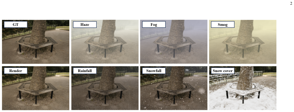
The load-bearing object is the explicit Gaussian primitive of 3D Gaussian Splatting, used not only to represent the reconstructed scene but as the unit of weather. During training the authors render depth and normal maps from the Gaussians, taking each Gaussian's shortest axis as its local normal, and supervise them with pseudo ground truth from a monocular depth estimator. After training, static weather is a depth-dependent alpha blend; dynamic weather is a separate point cloud of noise Gaussians rendered in sub-layers and composited through depth, brightness, distance, and color masks; snow accumulation is chosen by upward normals and densified on locally estimated planes.
What would settle it
Take a reconstructed scene with known planar surfaces, such as a wall, a ground plane, and a roof, and compare the direction of each Gaussian's shortest axis with the true surface normal obtained from LiDAR or the reconstruction itself. If the angular error is large for surfaces seen at oblique angles, the normal-consistency loss is not actually supervising geometry. A simpler check: render snow accumulation on a scene containing a vertical wall and a horizontal surface; if snow appears on the wall or fails to cover the horizontal surface, the shortest-axis normal assumption is falsified.
Extended reading notes
Core claim
The paper claims that weather simulation for real scenes does not require reconstructing the weathered scene or applying a generative image model; instead, it can be achieved by attaching Gaussian-based weather layers to an optimized clear-weather 3D Gaussian Splatting scene. Static weather is treated as a depth-dependent blending of the rendered image with a fog color, so the blur follows scene geometry. Dynamic weather is modeled as separate point clouds of noise Gaussians, rendered independently and composited through masks based on depth, brightness, distance, and color thresholds; partitioning the noise cloud into sub-layers avoids incorrect occlusion when multiple particles project to the same pixel. Snow accumulation is produced by selecting Gaussians whose shortest-axis normal points upward, densifying them on locally fitted planes, and filtering outliers. The authors state that this yields view-consistent, time-consistent, controllable weather synthesis with real-time rendering.
Load-bearing premise
The whole geometric pipeline relies on the assumption that a Gaussian's shortest axis points along the local surface normal, and the paper does not test this on varied geometry; if that link breaks, the normal-consistency loss and the placement of accumulated snow lose their grounding.
Editorial extensions
If this is right
- If this is right, anyone with a reconstructed 3D Gaussian scene can synthesize fog, haze, rain, snow, and snow accumulation without manual modeling or GPU-heavy diffusion, making interactive weather editing practical.
- Static weather rendering becomes depth-aware in real time, so near and far object boundaries remain distinct rather than being covered by a flat mask.
- Falling rain and snow remain consistent across frames and viewpoints because particles are explicit Gaussians with per-frame displacements, enabling coherent video instead of per-frame style transfer.
- Snow accumulation respects scene geometry via normal direction and local plane fitting, avoiding the depth-estimation failures seen in neural-radiance-field-based baselines.
- The synthesized outputs can serve as corner-case training data for perception systems in autonomous driving and aerial monitoring.
Reading between the lines
- Editorial inference: because each weather effect is a layer over the same reconstructed scene, the framework should support seamless interpolation between weather types by smoothly varying intensity, particle density, and color parameters; the paper does not test this.
- Editorial inference: the falling-particle model is kinematic rather than physical. Adding wind fields, collisions, or raindrop splashes would be a natural next step, and the explicit Gaussian representation makes such forces straightforward to attach, but the paper does not claim this.
- Editorial inference: a direct stress test would be to hold out real weather videos with ground-truth geometry and measure whether simulated weather changes the measured geometry or only the appearance, which would separate synthesis quality from the shortest-axis normal assumption.
Editorial analysis
A structured set of objections, weighed in public.
Referee Report
Summary. The paper proposes Weather-Magician, a 3D Gaussian Splatting-based framework that reconstructs clear-weather scenes and renders them with synthesized weather effects: static effects (fog, haze, smog) via depth-based post-processing, dynamic effects (rain, snowfall) via separately rendered Gaussian noise layers with depth and brightness masking, and cumulative effects (snow accumulation) via normal-based placement and plane densification. The authors report real-time frame rates on an RTX 4090 and compare qualitatively and quantitatively against ClimateGAN, Stable Diffusion, DID-MDN, and ClimateNeRF using the CMMD and UVQ metrics on real weather datasets.
Significance. The motivation is practical and the high-level architecture is sensible: weather elements are modeled explicitly as Gaussians, which makes the approach cheap, controllable, and naturally view-consistent. The paper includes honest discussion of limitations and provides concrete timing measurements, which are useful. However, the central claims of realism and controllability are not yet established: the key dynamic-weather blending formula (Eq. 14) is mathematically wrong as written, the shortest-axis-as-normal assumption is unverified and load-bearing, and the quantitative evidence is mixed rather than uniformly favorable. With corrections and additional evidence, the framework could be a valuable contribution.
major comments (4)
- [Section III-D, Eq. (14)] The luminance blending factor is defined as f_p^l = exp(min(max(L_sky - L_p, t_max), t_min)) - 1. Since max(x, t_max) is always at least t_max, and the text implies t_min <= t_max (t_min is negative for snow, t_max is 'moderate'), the inner min collapses the entire expression to exp(t_min) - 1 for every pixel. Consequently the brightness-dependent transparency mechanism described around Eqs. (11) and (16), and the controllability example in Fig. 11b, do not follow from the formula as written. This is load-bearing for the dynamic-weather realism and controllability claims. The intended expression appears to be exp(clamp(L_sky - L_p, t_min, t_max)) - 1, with clamp(x, a, b) = max(a, min(x, b)). Please correct the formula and either re-run the affected experiments or confirm that the implementation used the corrected version.
- [Section III-B and Section III-E] The paper states that 'we directly assign the shortest axis of each Gaussian as its corresponding normal vector' and then uses this normal both in the normal consistency loss (Eq. 7) and in deciding where accumulated snow should be placed (dot product with gravity in Section III-E). No evidence is provided that the shortest axis of an optimized 3D Gaussian reliably points along the local surface normal; for non-flat or tube-like Gaussians this is not generally true. Because errors in the normal directly corrupt the snow-cover geometry, please either add a shape regularizer that enforces flat, surface-aligned Gaussians, or provide a quantitative validation of the normal assumption, for example on a synthetic scene with known normals.
- [Section IV-J, Tables II and III] The claim that the method 'demonstrate[s] lower CMMD on both the static and dynamic weather simulation results' is not supported by the data. In the snow row, Ours (3.30) is worse than SD (2.66) and ClimateNeRF (2.96). The UVQ scores are also not uniformly higher, for example Garden fog is Ours 3.87 versus ClimateGAN 4.10, and Bicycle snow is Ours 3.79 versus SD 3.81. Moreover, the merged 'snow simulation' category makes the comparison with ClimateNeRF unfair, since ClimateNeRF does not simulate snowfall. Please report error bars or significance tests, separate snowfall and snow-accumulation comparisons, and discuss the failure cases; otherwise the central realism claim remains supported mainly by unverifiable qualitative figures.
- [Sections III-C through III-E, reproducibility] The method depends on a large set of manually set constants (I_style, C_fog, t_min, t_max, t_D, t_C, k, d_max, it_N, and the number and scale of inserted noise Gaussians), but the paper does not provide a complete parameter table or code release. Only it_N = 6000 is given explicitly. Given that Eq. (14) is already ambiguous, a reader cannot re-implement the method or independently verify the reported FPS and quality numbers. Please provide a full parameter listing or, preferably, release the code.
minor comments (6)
- [Section II heading] The heading 'REALTEDWORKS' should be 'RELATED WORKS'.
- [Section III-E, Eq. (17)] The definition r_plane = median(R_n)/(1+2σ_n) is unusual and not explained; if R_n is a set of distances, please clarify the intended statistic and define σ_n explicitly.
- [Table I] The table formatting is broken, with entries like 'ClimateGAN [42]\0.11\ \' and several empty cells; please reformat the table so the FPS values are readable.
- [Section IV-H] The sentence 'We validate the viewpoint consistency of our method through both qualitative experiments' is awkward and only one qualitative comparison is shown; please revise and, ideally, add a quantitative cross-view consistency measure.
- [Equations (11) and (16)] The notation for the noise layer and the blending factor is inconsistent (C_noise versus C^i_noise, f^l versus f_i^l); please define each symbol once and use it consistently.
- [Section III-D] The mechanism for temporal consistency is described only as adding different displacement to each noise Gaussian; please specify how displacements are sampled and how inter-frame coherence is enforced, since the 4D claim depends on it.
Circularity Check
No significant circularity: the weather effects are constructed from explicit geometry and external priors, with benchmarks used only for evaluation.
full rationale
The paper's central derivation is self-contained: weather effects are produced by explicit post-processing and Gaussian insertion rules driven by rendered depth/normal maps and user-set parameters (Eqs. 9-16). The depth prior from Depth Anything is an external supervision signal, and the CMMD/UVQ benchmarks are used only as after-the-fact evaluation, not as optimization targets. No claim is justified by a self-citation chain; references such as DNGaussian and 3DGS are external prior works. The shortest-axis-as-normal assumption in Section III-B is a geometric approximation and a correctness risk, not a circular definition, because the snow-placement rule uses the same normal but does not define the reconstruction target. The corrupted clamp in Eq. 14 is a correctness bug that would flatten the luminance factor, but it is not a reduction of the claimed result to an input. Accordingly, no circular step is exhibited.
Assumptions & free parameters
free parameters (8)
- I_style
- C_fog
- t_min, t_max
- t_D
- t_C
- k and sub-layer capacity
- d_max
- it_N =
6000
assumptions (6)
- standard math 3D Gaussian Splatting representation and alpha blending equations are correct and applicable.
- domain assumption Depth Anything's relative depth estimates reliably serve as pseudo ground truth for depth supervision.
- domain assumption The shortest axis of each Gaussian approximates the local surface normal.
- domain assumption Fog particles are uniformly distributed in space, so visibility follows an exponential falloff with depth.
- domain assumption Snow accumulates only on surfaces whose normals point upward within pi/6 of the gravity direction.
- ad hoc to paper Manually adding an upper hemisphere point cover to the initialized point cloud provides a correct sky prior.
Cite this review
Pith. "Pith review of Weather-Magician: Reconstruction and Rendering Framework for 4D Weather Synthesis In Real Time." pith.science (2026). https://pith.science/paper/7MBUBV6Y
@misc{pith2026250519919,
  author       = {Pith},
  title        = {Pith review of: Weather-Magician: Reconstruction and Rendering Framework for 4D Weather Synthesis In Real Time},
  year         = {2026},
  howpublished = {\url{https://pith.science/paper/7MBUBV6Y}},
  note         = {Machine review of arXiv:2505.19919}
}
read the original abstract
For tasks such as urban digital twins, VR/AR/game scene design, or creating synthetic films, the traditional industrial approach often involves manually modeling scenes and using various rendering engines to complete the rendering process. This approach typically requires high labor costs and hardware demands, and can result in poor quality when replicating complex real-world scenes. A more efficient approach is to use data from captured real-world scenes, then apply reconstruction and rendering algorithms to quickly recreate the authentic scene. However, current algorithms are unable to effectively reconstruct and render real-world weather effects. To address this, we propose a framework based on gaussian splatting, that can reconstruct real scenes and render them under synthesized 4D weather effects. Our work can simulate various common weather effects by applying Gaussians modeling and rendering techniques. It supports continuous dynamic weather changes and can easily control the details of the effects. Additionally, our work has low hardware requirements and achieves real-time rendering performance. The result demos can be accessed on our project homepage: weathermagician.github.io
Figures


Figures from the paper (7 more)


Forward citations
Cited by 1 Pith paper
-
muSync-GS: Physics-Synchronized Driving Video Synthesis for Weather and Geometric Road Hazards
muSync-GS couples weather and road-shape edits in driving videos to a calibrated vehicle-dynamics model, so the synthesized ego motion and telemetry change with the same controls that drive the visual edits.
Reference graph
Works this paper leans on
-
[1]
B. O. Community,Blender - a 3D modelling and ren- dering package, Blender Foundation, Stichting Blender Foundation, Amsterdam, 2018. [Online]. Available: http: //www.blender.org
work page 2018
-
[2]
Carla: An open urban driving simulator,
A. Dosovitskiy, G. Ros, F. Codevilla, A. Lopez, and V . Koltun, “Carla: An open urban driving simulator,” in Conference on robot learning. PMLR, 2017, pp. 1–16
work page 2017
-
[3]
Air- sim: High-fidelity visual and physical simulation for autonomous vehicles,
S. Shah, D. Dey, C. Lovett, and A. Kapoor, “Air- sim: High-fidelity visual and physical simulation for autonomous vehicles,” inField and Service Robotics: Results of the 11th International Conference. Springer, 2018, pp. 621–635. Fig. 11.Controllability. aproves the possibility to modify the intensity when applying blurring effect.bshows the different tra...
work page 2018
-
[4]
Knowledge-based virtual outdoor weather event simulator using unity 3d,
H. Noueihed, H. Harb, and J. Tekli, “Knowledge-based virtual outdoor weather event simulator using unity 3d,” The Journal of Supercomputing, vol. 78, no. 8, pp. 10 620–10 655, 2022
work page 2022
-
[5]
U. Engine, “Unreal engine,”Retrieved from Unreal 11 Engine: https://www. unrealengine. com/en-US/what-is- unreal-engine-4, 2018
work page 2018
-
[6]
Structure-from- motion revisited,
J. L. Schonberger and J.-M. Frahm, “Structure-from- motion revisited,” inProceedings of the IEEE conference on computer vision and pattern recognition, 2016, pp. 4104–4113
work page 2016
-
[7]
M. Goesele, B. Curless, and S. M. Seitz, “Multi-view stereo revisited,” in2006 IEEE Computer Society Con- ference on Computer Vision and Pattern Recognition (CVPR’06), vol. 2. IEEE, 2006, pp. 2402–2409
work page 2006
-
[8]
Nerf: Representing scenes as neural radiance fields for view synthesis,
B. Mildenhall, P. P. Srinivasan, M. Tancik, J. T. Barron, R. Ramamoorthi, and R. Ng, “Nerf: Representing scenes as neural radiance fields for view synthesis,”Communi- cations of the ACM, vol. 65, no. 1, pp. 99–106, 2021
work page 2021
Show all 47 references
-
[9]
3d gaussian splatting for real-time radiance field ren- dering
B. Kerbl, G. Kopanas, T. Leimk ¨uhler, and G. Drettakis, “3d gaussian splatting for real-time radiance field ren- dering.”ACM Trans. Graph., vol. 42, no. 4, pp. 139–1, 2023
2023
-
[10]
4d gaussian splatting for real- time dynamic scene rendering,
G. Wu, T. Yi, J. Fang, L. Xie, X. Zhang, W. Wei, W. Liu, Q. Tian, and X. Wang, “4d gaussian splatting for real- time dynamic scene rendering,” inProceedings of the IEEE/CVF Conference on Computer Vision and Pattern Recognition, 2024, pp. 20 310–20 320
2024
-
[11]
Weathergs: 3d scene reconstruction in adverse weather conditions via gaussian splatting,
C. Qian, Y . Guo, W. Li, and G. Markkula, “Weathergs: 3d scene reconstruction in adverse weather conditions via gaussian splatting,”arXiv preprint arXiv:2412.18862, 2024
2024 arXiv
-
[12]
Deraings: Gaussian splatting for enhanced scene reconstruction in rainy environments,
S. Liu, X. Chen, H. Chen, Q. Xu, and M. Li, “Deraings: Gaussian splatting for enhanced scene reconstruction in rainy environments,”arXiv preprint arXiv:2408.11540, 2024
2024 arXiv
-
[13]
Gaussianeditor: Editing 3d gaussians delicately with text instructions,
J. Wang, J. Fang, X. Zhang, L. Xie, and Q. Tian, “Gaussianeditor: Editing 3d gaussians delicately with text instructions,” inProceedings of the IEEE/CVF Confer- ence on Computer Vision and Pattern Recognition, 2024, pp. 20 902–20 911
2024
-
[14]
View-consistent 3d editing with gaussian splatting,
Y . Wang, X. Yi, Z. Wu, N. Zhao, L. Chen, and H. Zhang, “View-consistent 3d editing with gaussian splatting,” in European Conference on Computer Vision. Springer, 2025, pp. 404–420
2025
-
[15]
Texture-gs: Disentangling the geometry and texture for 3d gaussian splatting editing,
T.-X. Xu, W. Hu, Y .-K. Lai, Y . Shan, and S.-H. Zhang, “Texture-gs: Disentangling the geometry and texture for 3d gaussian splatting editing,” inEuropean Conference on Computer Vision. Springer, 2025, pp. 37–53
2025
-
[16]
Gstex: Per-primitive texturing of 2d gaus- sian splatting for decoupled appearance and geometry modeling,
V . Rong, J. Chen, S. Bahmani, K. N. Kutulakos, and D. B. Lindell, “Gstex: Per-primitive texturing of 2d gaus- sian splatting for decoupled appearance and geometry modeling,”arXiv preprint arXiv:2409.12954, 2024
2024 arXiv
-
[17]
Dge: Direct gaussian 3d editing by consistent multi-view editing,
M. Chen, I. Laina, and A. Vedaldi, “Dge: Direct gaussian 3d editing by consistent multi-view editing,” inEuropean Conference on Computer Vision. Springer, 2024, pp. 74–92
2024
-
[18]
Rainygs: Efficient rain synthesis with physically-based gaussian splatting,
Q. Dai, X. Ni, Q. Shen, W. Chen, B. Chen, and M. Chu, “Rainygs: Efficient rain synthesis with physically-based gaussian splatting,”arXiv preprint arXiv:2503.21442, 2025
2025 arXiv
-
[19]
Let it snow! animating static gaussian scenes with dynamic weather effects,
G. Fiebelman, H. Averbuch-Elor, and S. Benaim, “Let it snow! animating static gaussian scenes with dynamic weather effects,”arXiv preprint arXiv:2504.05296, 2025
2025
-
[20]
Gaussctrl: Multi-view consistent text-driven 3d gaussian splatting editing,
J. Wu, J.-W. Bian, X. Li, G. Wang, I. Reid, P. Torr, and V . A. Prisacariu, “Gaussctrl: Multi-view consistent text-driven 3d gaussian splatting editing,” inEuropean Conference on Computer Vision. Springer, 2024, pp. 55–71
2024
-
[21]
Denoising diffusion probabilistic models,
J. Ho, A. Jain, and P. Abbeel, “Denoising diffusion probabilistic models,”Advances in neural information processing systems, vol. 33, pp. 6840–6851, 2020
2020
-
[22]
Simulating photo-realistic snow and fog on existing images for enhanced cnn training and evaluation,
A. V on Bernuth, G. V olk, and O. Bringmann, “Simulating photo-realistic snow and fog on existing images for enhanced cnn training and evaluation,” in2019 IEEE Intelligent Transportation Systems Conference (ITSC). IEEE, 2019, pp. 41–46
2019
-
[23]
Digiweather: Synthetic rain, snow and fog dataset augmentation,
I. Nikolov, “Digiweather: Synthetic rain, snow and fog dataset augmentation,” inInternational Conference on Extended Reality. Springer, 2024, pp. 22–41
2024
-
[24]
Generative adversarial networks,
I. Goodfellow, J. Pouget-Abadie, M. Mirza, B. Xu, D. Warde-Farley, S. Ozair, A. Courville, and Y . Bengio, “Generative adversarial networks,”Communications of the ACM, vol. 63, no. 11, pp. 139–144, 2020
2020
-
[25]
Style- bank: An explicit representation for neural image style transfer,
D. Chen, L. Yuan, J. Liao, N. Yu, and G. Hua, “Style- bank: An explicit representation for neural image style transfer,” inProceedings of the IEEE conference on computer vision and pattern recognition, 2017, pp. 1897– 1906
2017
-
[26]
Style transfer for anime sketches with enhanced residual u-net and auxil- iary classifier gan,
L. Zhang, Y . Ji, X. Lin, and C. Liu, “Style transfer for anime sketches with enhanced residual u-net and auxil- iary classifier gan,” in2017 4th IAPR Asian conference on pattern recognition (ACPR). IEEE, 2017, pp. 506– 511
2017
-
[27]
Stylediffusion: Control- lable disentangled style transfer via diffusion models,
Z. Wang, L. Zhao, and W. Xing, “Stylediffusion: Control- lable disentangled style transfer via diffusion models,” in Proceedings of the IEEE/CVF International Conference on Computer Vision, 2023, pp. 7677–7689
2023
-
[28]
Weather gan: Multi- domain weather translation using generative adversarial networks,
X. Li, K. Kou, and B. Zhao, “Weather gan: Multi- domain weather translation using generative adversarial networks,”arXiv preprint arXiv:2103.05422, 2021
2021 arXiv
-
[29]
Weatherdg: Llm-assisted procedural weather generation for domain- generalized semantic segmentation,
C. Qian, Y . Guo, Y . Mo, and W. Li, “Weatherdg: Llm-assisted procedural weather generation for domain- generalized semantic segmentation,”arXiv preprint arXiv:2410.12075, 2024
2024 arXiv
-
[30]
Deepcache: Acceler- ating diffusion models for free,
X. Ma, G. Fang, and X. Wang, “Deepcache: Acceler- ating diffusion models for free,” inProceedings of the IEEE/CVF conference on computer vision and pattern recognition, 2024, pp. 15 762–15 772
2024
-
[31]
Speed is all you need: On-device acceleration of large diffusion models via gpu- aware optimizations,
Y .-H. Chen, R. Sarokin, J. Lee, J. Tang, C.-L. Chang, A. Kulik, and M. Grundmann, “Speed is all you need: On-device acceleration of large diffusion models via gpu- aware optimizations,” inProceedings of the IEEE/CVF Conference on Computer Vision and Pattern Recognition, 2023,...
2023
-
[32]
Fastercache: Training-free video diffusion model acceleration with high quality,
Z. Lv, C. Si, J. Song, Z. Yang, Y . Qiao, Z. Liu, and K.- Y . K. Wong, “Fastercache: Training-free video diffusion model acceleration with high quality,”arXiv preprint arXiv:2410.19355, 2024
2024 arXiv
-
[33]
Climatenerf: Extreme weather synthesis in neural ra- 12 diance field,
Y . Li, Z.-H. Lin, D. Forsyth, J.-B. Huang, and S. Wang, “Climatenerf: Extreme weather synthesis in neural ra- 12 diance field,” inProceedings of the IEEE/CVF Interna- tional Conference on Computer Vision, 2023, pp. 3227– 3238
2023
-
[34]
Styledstreets: Multi-style street simulator with spatial and temporal consistency,
Y . Chen, Y . Wang, X. Zhang, K. Zhan, P. Jia, Y . Zhan, and X. Lang, “Styledstreets: Multi-style street simulator with spatial and temporal consistency,”arXiv preprint arXiv:2503.21104, 2025
2025 arXiv
-
[35]
Depth anything: Unleashing the power of large-scale unlabeled data,
L. Yang, B. Kang, Z. Huang, X. Xu, J. Feng, and H. Zhao, “Depth anything: Unleashing the power of large-scale unlabeled data,” inProceedings of the IEEE/CVF Conference on Computer Vision and Pattern Recognition, 2024, pp. 10 371–10 381
2024
-
[36]
Dngaussian: Optimizing sparse-view 3d gaussian radiance fields with global-local depth normalization,
J. Li, J. Zhang, X. Bai, J. Zheng, X. Ning, J. Zhou, and L. Gu, “Dngaussian: Optimizing sparse-view 3d gaussian radiance fields with global-local depth normalization,” in Proceedings of the IEEE/CVF Conference on Computer Vision and Pattern Recognition, 2024, pp. 20 775–20 785
2024
-
[37]
Mip-nerf 360: Unbounded anti-aliased neural radiance fields,
J. T. Barron, B. Mildenhall, D. Verbin, P. P. Srinivasan, and P. Hedman, “Mip-nerf 360: Unbounded anti-aliased neural radiance fields,” inProceedings of the IEEE/CVF conference on computer vision and pattern recognition, 2022, pp. 5470–5479
2022
-
[38]
Seeing through fog without seeing fog: Deep multimodal sensor fusion in unseen adverse weather,
M. Bijelic, T. Gruber, F. Mannan, F. Kraus, W. Ritter, K. Dietmayer, and F. Heide, “Seeing through fog without seeing fog: Deep multimodal sensor fusion in unseen adverse weather,” inThe IEEE/CVF Conference on Com- puter Vision and Pattern Recognition (CVPR), June 2020
2020
-
[39]
Structure representation network and uncertainty feedback learning for dense non-uniform fog removal,
Y . Jin, W. Yan, W. Yang, and R. T. Tan, “Structure representation network and uncertainty feedback learning for dense non-uniform fog removal,” inAsian Conference on Computer Vision. Springer, 2022, pp. 155–172
2022
-
[40]
Benchmarking single-image dehazing and beyond,
B. Li, W. Ren, D. Fu, D. Tao, D. Feng, W. Zeng, and Z. Wang, “Benchmarking single-image dehazing and beyond,”IEEE Transactions on Image Processing, vol. 28, no. 1, pp. 492–505, 2019
2019
-
[41]
Single image deraining: A comprehensive benchmark analysis,
S. Li, I. B. Araujo, W. Ren, Z. Wang, E. K. Tokuda, R. H. Junior, R. Cesar-Junior, J. Zhang, X. Guo, and X. Cao, “Single image deraining: A comprehensive benchmark analysis,” inProceedings of the IEEE/CVF Conference on Computer Vision and Pattern Recognition, 2019, pp. 3838–3847
2019
-
[42]
Climategan: Raising climate change awareness by generating images of floods,
V . Schmidt, A. S. Luccioni, M. Teng, T. Zhang, A. Rey- naud, S. Raghupathi, G. Cosne, A. Juraver, V . Vardanyan, A. Hernandez-Garciaet al., “Climategan: Raising climate change awareness by generating images of floods,”arXiv preprint arXiv:2110.02871, 2021
-
[43]
High-resolution image synthesis with la- tent diffusion models,
R. Rombach, A. Blattmann, D. Lorenz, P. Esser, and B. Ommer, “High-resolution image synthesis with la- tent diffusion models,” inProceedings of the IEEE/CVF conference on computer vision and pattern recognition, 2022, pp. 10 684–10 695
2022
-
[44]
Density-aware single image de-raining using a multi-stream dense network,
H. Zhang and V . M. Patel, “Density-aware single image de-raining using a multi-stream dense network,” inPro- ceedings of the IEEE conference on computer vision and pattern recognition, 2018, pp. 695–704
2018
-
[45]
Rethinking fid: Towards a better evaluation metric for image generation,
S. Jayasumana, S. Ramalingam, A. Veit, D. Glasner, A. Chakrabarti, and S. Kumar, “Rethinking fid: Towards a better evaluation metric for image generation,” in Proceedings of the IEEE/CVF Conference on Computer Vision and Pattern Recognition, 2024, pp. 9307–9315
2024
-
[46]
Rich features for perceptual quality assessment of ugc videos,
Y . Wang, J. Ke, H. Talebi, J. G. Yim, N. Birkbeck, B. Adsumilli, P. Milanfar, and F. Yang, “Rich features for perceptual quality assessment of ugc videos,” in Proceedings of the IEEE/CVF conference on computer vision and pattern recognition, 2021, pp. 13 435–13 444
2021
-
[47]
Challenges, evaluation and opportunities for open- world learning,
M. Kejriwal, E. Kildebeck, R. Steininger, and A. Shrivas- tava, “Challenges, evaluation and opportunities for open- world learning,”Nature Machine Intelligence, vol. 6, no. 6, pp. 580–588, 2024
2024
Reviewed August 7, 2026 · model on record in the stance chip above.
Discussion (0). Continue with ORCID to comment.