REVIEW 5 major objections 7 minor 36 references
Spatiotemporal Causal Decoupling Model for Air Quality Forecasting
T0 review · 5 major / 7 minor · reviewed 2026-08-07 · deepseek-v4-flash
Pith's one-line read The paper claims that explicitly modeling causal links between weather and pollution history, then diffusing that knowledge through future weather inputs, yields over 20% relative improvement in air quality forecasting.
desk verdict A solid new architecture with strong KnowAir results, but the abstract overstates the margin and the 'causal' framing is mostly a label. read the letter →
The pith
A machine-rendered reading of the paper's core claim, the machinery that carries it, and where it could break.
The reading
What carries the argument
The key machinery is the air causal decoupling module, a pair of stacked DK-MSA attention layers: Cade (causal decoupling) as encoder and Cadi (causal diffusion) as decoder. DK-MSA computes attention from four paths, a scaled query-key product, a learnable adaptive adjacency pair, and their transposes, so the model can mix data-driven and learned station and time relations. Cade uses the historical meteorological representation as query and key and the AQI representation as value; Cadi uses the future meteorological representation as query and key and the decoupled output as value. A causal intervention mechanism then selects from K binary temporal and spatial masks the one that maximizes loss variance and minimizes that loss plus a regularizer, forcing the model to be robust to perturbed future weather inputs.
What would settle it
Train the identical AirCade model on a dataset that includes real operational weather forecasts rather than noise-corrupted observations, and compare its accuracy with the best baseline. If the reported margin disappears or drops below statistical significance under real forecast error, the causal intervention mechanism's contribution is an artifact of the Gaussian noise model.
Extended reading notes
Core claim
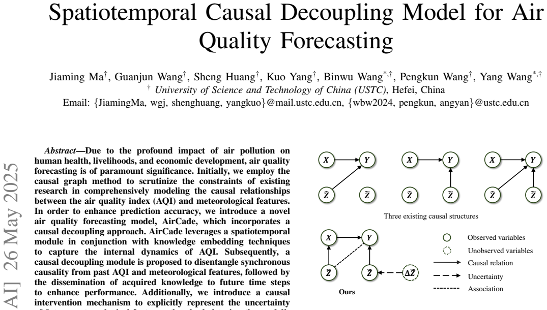
On the paper's own terms, the central discovery is that disentangling synchronous causality, how simultaneous weather drives AQI, from the AQI's own temporal dynamics is what lets a forecaster use future weather profitably. Existing models, the paper argues, fall into three causal structures that either concatenate AQI and weather as input channels or use shallow decoders; AirCade instead treats past weather as queries and keys reading AQI values in its causal decoupling layer, then treats future weather as queries and keys reading the resulting coupling in its causal diffusion layer. Together with attention masks chosen to maximize loss variance, this yields a model that is more accurate and more robust to noise in forecasted weather. The reported outcome is a new best on KnowAir, with MAE 14.60 (2015) and 11.29 (2017) versus 17.44 and 13.57 for the best baseline, plus higher critical success index and probability of detection and lower false alarm rate.
Load-bearing premise
The load-bearing premise is that corrupting future meteorological inputs with standard normal noise faithfully simulates the uncertainty of real weather forecasts; if actual forecast errors are correlated across stations or non-Gaussian, the reported robustness and accuracy gains may shrink in practice.
Editorial extensions
If this is right
- A new reported state of the art for 24-hour-ahead PM2.5 forecasting on KnowAir, with MAE 14.60 (2015) and 11.29 (2017) versus 17.44 and 13.57 for the best baseline.
- Future weather data helps most when it is routed through an attention pathway that reads a causal coupling representation, not when it is concatenated as extra input features.
- Domain-knowledge prompts, station identity, time-of-day, and day-of-week, improve spatiotemporal forecasting beyond learned representations alone.
- The intervention mechanism offers a template for training robust models when auxiliary inputs are uncertain: perturb attention masks and minimize worst-environment loss.
Reading between the lines
- A natural extension is to test AirCade's decoupling on traffic or energy forecasting, where exogenous future covariates such as weather or grid prices carry similar uncertainty; the causal decoupling pathway may transfer directly.
- The Gaussian-noise model for weather forecast error is the load-bearing simplification; replacing it with real forecast-error statistics or structured perturbations would reveal whether the robustness mechanism generalizes.
- The choice of mask that maximizes loss variance resembles invariant risk minimization; if so, AirCade may also improve out-of-distribution transfer across cities or seasons, which the paper does not directly test.
- Because the paper reports only two years of one dataset, a natural check is whether the margin persists across other years, seasons, or regions with different pollution regimes.
Signed reviews
Editorial analysis
A structured set of objections, weighed in public.
Referee Report
Summary. The paper proposes AirCade, a Transformer-based spatiotemporal model for hourly PM2.5 forecasting. AirCade embeds domain knowledge in the form of temporal, station, and positional prompts; uses paired Cade/Cadi attention layers to transfer past air quality and weather information to future predictions; and applies binary attention masks, selected by a bi-level objective, to simulate interventions on future weather uncertainty. Experiments on the KnowAir 2015 and 2017 subsets compare against 12 baselines and report MAEs of 14.60 and 11.29, respectively, with an abstract claim of over 20% relative improvement over state-of-the-art models.
Significance. If the reported results are reproducible, AirCade is a strong empirical result for nationwide PM2.5 forecasting, improving over DeepAir and Airformer on all metrics with standard deviations. The authors provide a source-code link and report error bars. However, the 20% claim is supported only by MAPE, not by MAE or RMSE, and the experiment omits several details needed for independent verification. The causal framing is mostly architectural, and the intervention experiment uses an idealized noise model, so the external validity of the robustness gains remains open.
major comments (5)
- [Abstract and Table I] The abstract states 'over 20% relative improvement' without specifying the metric. Using Table I, relative to the best baseline (DeepAir), the MAE gains are (17.44-14.60)/17.44 = 16.3% on KnowAir 2015 and (13.57-11.29)/13.57 = 16.8% on 2017; RMSE gains are about 13.5% on both years; only MAPE gains (25.2% and 26.0%) exceed 20%. The claim should be metric-specific and, if the intended metric is MAE, the percentage should be corrected. This is load-bearing because the stated margin is the basis for the state-of-the-art claim.
- [III-C, Eq. (13)] Equation (13) defines a bi-level problem in which M* = argmax_k Var{L(Y|M_k,Theta)} and the outer objective is minimized over Theta. The paper does not describe how this bi-level problem is solved, whether gradients flow through the argmax, how the finite set of K masks relates to all possible masks, or what value of beta is used. Without this, the causal intervention mechanism is underspecified and cannot be reproduced from the text. The hyperparameter section says 'Mask matrix number Ke' despite Eq. (13) using K, so the notation is also inconsistent.
- [IV-A and Footnote 1] Future meteorological features are simulated by adding standard normal noise to the observed future values. This assumes that forecast error is i.i.d. Gaussian with unit variance and is independent across stations and time steps. Real weather forecasts have structured, correlated, and non-Gaussian errors. The paper provides no sensitivity analysis over noise levels or distributions and no test with actual forecast data, so the claim that the intervention mechanism provides robustness in operational use is not supported.
- [IV-A, Experiment Setting] The experimental setup is incomplete. Section IV-A does not state the train/validation/test split (temporal ordering, ratio, or whether stations are held out), the normalization method, the embedding dimensions dP, dm, ds, the batch size, the number of training epochs, the value of beta in Eq. (13), or the loss function used. These details are needed to verify the reported standard deviations and to compare with baselines under identical conditions.
- [III and Fig. 1] The paper labels the approach 'causal' on the basis of the graph in Fig. 1, but it specifies no structural equations, no causal identification argument, and no test of the assumed graph. The Cade/Cadi modules are attention layers whose attention matrices are learned from data; the 'intervention' is binary masking of attention coefficients. Claims such as 'explicitly models the complex causal relationships' in the introduction therefore go beyond what the architecture establishes. I recommend either softening the causal language or adding a formal statement of which causal quantity is estimated and under what assumptions.
minor comments (7)
- [III-A] 'Then we integer embedded information into three variables' should read 'integrate'.
- [III-B2] 'it taks historical meteorological representation' contains a typo ('taks' for 'takes').
- [Table I] Several rows have run-together numbers; for example, the STAEformer row reads '89.27±1.5524.06±1.5314.59±0.60' with no separators. Please regenerate the table with clean formatting so each metric is unambiguously separated.
- [Figures 4 and 5] The axis labels and legend text in Figures 4 and 5 appear as unicode escape sequences, making the ablation and hyperparameter results unreadable. Replace them with readable text.
- [IV-A and Eq. (13)] The number of masking environments is denoted K in Eq. (13) but called 'Ke' in the hyperparameter discussion; the notation should be unified.
- [III-B1, Eq. (2)] Equation (2) uses [A1,A2,A3,A4] V, but the A_i are N×N matrices and V is N×d; please specify explicitly how the four attention matrices are combined (e.g., concatenation across heads or a sum).
- [Conclusion] 'a intervention mechanism' should be 'an intervention mechanism'.
Circularity Check
No circularity found: AirCade's predictions are produced by learned mappings from historical and future-weather inputs, with no fitted parameter or self-cited premise forcing the output.
full rationale
The paper's derivation chain is empirical and self-contained. Equation (12) computes the prediction Y_hat as a linear map of the learned representation O_tilde_L2, which itself is produced by the transformer stacks (Eqs. 8-11) from the input AQI history X, past weather Z_hat, and future weather Z_tilde. No parameter is defined in terms of the target Y, and no quantity is fitted to the reported metric and then reported as a prediction. The causal intervention objective (Eq. 13) is a min-max training loss over masks M, and the future-weather uncertainty is simulated by adding standard normal noise to Z_tilde (Section IV-A1); neither step makes the output equal to an input or to a fitted value. The self-citations (e.g., Refs. [8], [9], [14]-[16], [25], [26]) motivate general spatiotemporal techniques but are not load-bearing for the central forecasting result; the performance comparison in Table I is against external baselines with reported numbers. The abstract's 'over 20% relative improvement' is metric-dependent: only MAPE exceeds 20% (25.2% and 26.0%), while MAE improvements are about 16.3% and 16.8%, and RMSE improvements about 13.5%. This is an accuracy/overstatement concern, not circularity, because the underlying experiments are independent of the claim's wording. Overall, no step in the paper reduces by construction to its own inputs.
Assumptions & free parameters
free parameters (5)
- Noise distribution for future weather =
N(0,1)
- Number of transformer layers L1, L2 =
3, 3
- Head number Kh and environment number K =
8, 3
- Balance coefficient beta =
not stated
- Embedding dimensions eD, eS, eP =
not stated
assumptions (4)
- domain assumption The causal graph in Fig. 1 with arrows from past AQI and weather to future AQI, plus unobserved variables, is the true data-generating process.
- ad hoc to paper Causal intervention can be implemented by binary masking of attention coefficients.
- domain assumption Future meteorological features are available as model inputs (or can be simulated with noise).
- domain assumption The KnowAir dataset with 184 cities is representative and the reported train/test protocol is followed consistently for all baselines.
Cite this review
Pith. "Pith review of Spatiotemporal Causal Decoupling Model for Air Quality Forecasting." pith.science (2026). https://pith.science/paper/LOZOFSMA
@misc{pith2026250520119,
  author       = {Pith},
  title        = {Pith review of: Spatiotemporal Causal Decoupling Model for Air Quality Forecasting},
  year         = {2026},
  howpublished = {\url{https://pith.science/paper/LOZOFSMA}},
  note         = {Machine review of arXiv:2505.20119}
}
read the original abstract
Due to the profound impact of air pollution on human health, livelihoods, and economic development, air quality forecasting is of paramount significance. Initially, we employ the causal graph method to scrutinize the constraints of existing research in comprehensively modeling the causal relationships between the air quality index (AQI) and meteorological features. In order to enhance prediction accuracy, we introduce a novel air quality forecasting model, AirCade, which incorporates a causal decoupling approach. AirCade leverages a spatiotemporal module in conjunction with knowledge embedding techniques to capture the internal dynamics of AQI. Subsequently, a causal decoupling module is proposed to disentangle synchronous causality from past AQI and meteorological features, followed by the dissemination of acquired knowledge to future time steps to enhance performance. Additionally, we introduce a causal intervention mechanism to explicitly represent the uncertainty of future meteorological features, thereby bolstering the model's robustness. Our evaluation of AirCade on an open-source air quality dataset demonstrates over 20\% relative improvement over state-of-the-art models.
Figures


Figures from the paper (3 more)


Reference graph
Works this paper leans on
-
[1]
D. A. Vallero, Fundamentals of air pollution . Academic press, 2014
work page 2014
-
[2]
Federated graph learning under domain shift with generalizable prototypes,
G. Wan, W. Huang, and M. Ye, “Federated graph learning under domain shift with generalizable prototypes,” in Proceedings of the AAAI Conference on Artificial Intelligence , vol. 38, pp. 15429–15437, 2024
work page 2024
-
[3]
LOHA: Direct Graph Spectral Contrastive Learning Between Low-pass and High-pass Views
Z. Zou, Y . Jiang, L. Shen, J. Liu, and X. Liu, “Loha: Direct graph spectral contrastive learning between low-pass and high-pass views,” arXiv preprint arXiv:2501.02969 , 2025
work page Pith review arXiv 2025
-
[4]
Epidemiology-Aware Neural ODE with Continuous Disease Transmission Graph
G. Wan, Z. Liu, M. S. Lau, B. A. Prakash, and W. Jin, “Epidemiology- aware neural ode with continuous disease transmission graph,” arXiv preprint arXiv:2410.00049, 2024
work page Pith review arXiv 2024
-
[5]
Crossgnn: Confronting noisy multivariate time series via cross interaction refinement,
Q. Huang, L. Shen, R. Zhang, S. Ding, B. Wang, Z. Zhou, and Y . Wang, “Crossgnn: Confronting noisy multivariate time series via cross interaction refinement,” Advances in Neural Information Processing Systems, vol. 36, pp. 46885–46902, 2023
work page 2023
-
[6]
Improving generalization of dynamic graph learning via environment prompt,
K. Yang, Z. Zhou, Q. Huang, L. Li, Y . Liang, and Y . Wang, “Improving generalization of dynamic graph learning via environment prompt,” in The Thirty-eighth Annual Conference on Neural Information Processing Systems
-
[7]
L. Chen, J. Fang, T. Liu, F. Gao, and L. Wang, “Stcontext: A mul- tifaceted dataset for developing context-aware spatio-temporal crowd mobility prediction models,” arXiv preprint arXiv:2501.03583 , 2025
work page Pith review arXiv 2025
-
[8]
Pattern expansion and consolidation on evolving graphs for continual traffic prediction,
B. Wang, Y . Zhang, X. Wang, P. Wang, Z. Zhou, L. Bai, and Y . Wang, “Pattern expansion and consolidation on evolving graphs for continual traffic prediction,” in Proceedings of the 29th ACM SIGKDD Conference on Knowledge Discovery and Data Mining , pp. 2223–2232, 2023
work page 2023
Show all 36 references
-
[9]
Knowledge expansion and consolidation for continual traffic prediction with expanding graphs,
B. Wang, Y . Zhang, J. Shi, P. Wang, X. Wang, L. Bai, and Y . Wang, “Knowledge expansion and consolidation for continual traffic prediction with expanding graphs,” IEEE Transactions on Intelligent Transporta- tion Systems, 2023
2023
-
[10]
A unified replay-based continuous learning framework for spatio-temporal prediction on streaming data,
H. Miao, Y . Zhao, C. Guo, B. Yang, Z. Kai, F. Huang, J. Xie, and C. S. Jensen, “A unified replay-based continuous learning framework for spatio-temporal prediction on streaming data,” in ICDE, 2024
2024
-
[11]
Expand and compress: Exploring tuning prin- ciples for continual spatio-temporal graph forecasting,
W. Chen and Y . Liang, “Expand and compress: Exploring tuning prin- ciples for continual spatio-temporal graph forecasting,” arXiv preprint arXiv:2410.12593, 2024
2024
-
[12]
A dynamic hypergraph attention network: Capturing market-wide spatiotemporal dependencies for stock selection,
Z. Liu, P. Duan, X. Xue, C. Zhang, W. Yue, and B. Zhang, “A dynamic hypergraph attention network: Capturing market-wide spatiotemporal dependencies for stock selection,” Applied Soft Computing , p. 112524, 2024
2024
-
[13]
Modeling spatio-temporal mobility across data silos via personalized federated learning,
Y . Zhang, X. Wang, P. Wang, B. Wang, Z. Zhou, and Y . Wang, “Modeling spatio-temporal mobility across data silos via personalized federated learning,” IEEE Transactions on Mobile Computing , 2024
2024
-
[14]
Stone: A spatio-temporal ood learning framework kills both spatial and temporal shifts,
B. Wang, J. Ma, P. Wang, X. Wang, Y . Zhang, Z. Zhou, and Y . Wang, “Stone: A spatio-temporal ood learning framework kills both spatial and temporal shifts,” in Proceedings of the 30th ACM SIGKDD Conference on Knowledge Discovery and Data Mining , pp. 2948–2959, 2024
2024
-
[15]
Towards dynamic spatial-temporal graph learning: A decoupled per- spective,
B. Wang, P. Wang, Y . Zhang, X. Wang, Z. Zhou, L. Bai, and Y . Wang, “Towards dynamic spatial-temporal graph learning: A decoupled per- spective,” in Proceedings of the AAAI Conference on Artificial Intelli- gence, vol. 38, pp. 9089–9097, 2024
2024
-
[16]
Meta koopman decomposition for time series forecasting under tem- poral distribution shifts,
Y . Zhang, X. Wang, Z. Sun, P. Wang, B. Wang, L. Li, and Y . Wang, “Meta koopman decomposition for time series forecasting under tem- poral distribution shifts,” Advanced Engineering Informatics , vol. 62, p. 102840, 2024
2024
-
[17]
Pm2. 5- gnn: A domain knowledge enhanced graph neural network for pm2. 5 forecasting,
S. Wang, Y . Li, J. Zhang, Q. Meng, L. Meng, and F. Gao, “Pm2. 5- gnn: A domain knowledge enhanced graph neural network for pm2. 5 forecasting,” in Proceedings of the 28th international conference on advances in geographic information systems , pp. 163–166, 2020
2020
-
[18]
Airformer: Predicting nationwide air quality in china with transformers,
Y . Liang, Y . Xia, S. Ke, Y . Wang, Q. Wen, J. Zhang, Y . Zheng, and R. Zimmermann, “Airformer: Predicting nationwide air quality in china with transformers,” in Proceedings of the AAAI Conference on Artificial Intelligence, vol. 37, pp. 14329–14337, 2023
2023
-
[19]
Decoupled dynamic spatial-temporal graph neural network for traffic forecasting,
Z. Shao, Z. Zhang, W. Wei, F. Wang, Y . Xu, X. Cao, and C. S. Jensen, “Decoupled dynamic spatial-temporal graph neural network for traffic forecasting,” Proc. VLDB Endow., vol. 15, no. 11, pp. 2733–2746, 2022
2022
-
[20]
Pdformer: Propagation delay-aware dynamic long-range transformer for traffic flow prediction,
J. Jiang, C. Han, W. X. Zhao, and J. Wang, “Pdformer: Propagation delay-aware dynamic long-range transformer for traffic flow prediction,” in Proceedings of the AAAI conference on artificial intelligence , vol. 37, pp. 4365–4373, 2023
2023
-
[21]
Visual prompt tuning,
M. Jia, L. Tang, B.-C. Chen, C. Cardie, S. Belongie, B. Hariharan, and S.-N. Lim, “Visual prompt tuning,” in European Conference on Computer Vision, pp. 709–727, Springer, 2022
2022
-
[22]
Attention is all you need,
A. Vaswani, N. Shazeer, N. Parmar, J. Uszkoreit, L. Jones, A. N. Gomez, Ł. Kaiser, and I. Polosukhin, “Attention is all you need,” Advances in neural information processing systems , vol. 30, 2017
2017
-
[23]
Informer: Beyond efficient transformer for long sequence time-series forecasting,
H. Zhou, S. Zhang, J. Peng, S. Zhang, J. Li, H. Xiong, and W. Zhang, “Informer: Beyond efficient transformer for long sequence time-series forecasting,” in Proceedings of the AAAI conference on artificial intel- ligence, vol. 35, pp. 11106–11115, 2021
2021
-
[24]
Divide the gradient by a running average of its recent magnitude. coursera: Neural networks for machine learning,
T. Tieleman and G. Hinton, “Divide the gradient by a running average of its recent magnitude. coursera: Neural networks for machine learning,” Technical report, 2017
2017
-
[25]
Condition-guided urban traffic co-prediction with multiple sparse surveillance data,
B. Wang, P. Wang, Y . Zhang, X. Wang, Z. Zhou, and Y . Wang, “Condition-guided urban traffic co-prediction with multiple sparse surveillance data,” IEEE Transactions on Vehicular Technology, 2024
2024
-
[26]
Get rid of isolation: A continuous multi-task spatio-temporal learning frame- work,
Z. Yi, Z. Zhou, Q. Huang, Y . Chen, L. Yu, X. Wang, and Y . Wang, “Get rid of isolation: A continuous multi-task spatio-temporal learning frame- work,” in The Thirty-eighth Annual Conference on Neural Information Processing Systems
-
[27]
Spatial-temporal identity: A simple yet effective baseline for multivariate time series forecasting,
Z. Shao, Z. Zhang, F. Wang, W. Wei, and Y . Xu, “Spatial-temporal identity: A simple yet effective baseline for multivariate time series forecasting,” in Proceedings of the 31st ACM International Conference on Information & Knowledge Management , pp. 4454–4458, 2022
2022
-
[28]
Spatio-temporal graph convolutional networks: A deep learning framework for traffic forecasting,
B. Yu, H. Yin, and Z. Zhu, “Spatio-temporal graph convolutional networks: A deep learning framework for traffic forecasting,” arXiv preprint arXiv:1709.04875, 2017
2017 arXiv
-
[29]
Graph wavenet for deep spatial-temporal graph modeling,
Z. Wu, S. Pan, G. Long, J. Jiang, and C. Zhang, “Graph wavenet for deep spatial-temporal graph modeling,” arXiv preprint arXiv:1906.00121 , 2019
1906 arXiv
-
[30]
Deciphering spatio-temporal graph forecasting: A causal lens and treatment,
Y . Xia, Y . Liang, H. Wen, X. Liu, K. Wang, Z. Zhou, and R. Zimmer- mann, “Deciphering spatio-temporal graph forecasting: A causal lens and treatment,” Advances in Neural Information Processing Systems , vol. 36, 2024
2024
-
[31]
Spatio-temporal adaptive embedding makes vanilla transformer sota for traffic forecasting,
H. Liu, Z. Dong, R. Jiang, J. Deng, J. Deng, Q. Chen, and X. Song, “Spatio-temporal adaptive embedding makes vanilla transformer sota for traffic forecasting,” in Proceedings of the 32nd ACM international conference on information and knowledge management , pp. 4125–4129, 2023
2023
-
[32]
Spatial-temporal transformer networks for traffic flow forecasting,
M. Xu, W. Dai, C. Liu, X. Gao, W. Lin, G.-J. Qi, and H. Xiong, “Spatial-temporal transformer networks for traffic flow forecasting,” arXiv preprint arXiv:2001.02908 , 2020
2001 arXiv
-
[33]
A hybrid model for spa- tiotemporal forecasting of pm2. 5 based on graph convolutional neural network and long short-term memory,
Y . Qi, Q. Li, H. Karimian, and D. Liu, “A hybrid model for spa- tiotemporal forecasting of pm2. 5 based on graph convolutional neural network and long short-term memory,”Science of the Total Environment, vol. 664, pp. 1–10, 2019
2019
-
[34]
Group-aware graph neural network for nationwide city air quality forecasting,
L. Chen, J. Xu, B. Wu, and J. Huang, “Group-aware graph neural network for nationwide city air quality forecasting,” ACM Transactions on Knowledge Discovery from Data , vol. 18, no. 3, pp. 1–20, 2023
2023
-
[35]
Deep distributed fusion network for air quality prediction,
X. Yi, J. Zhang, Z. Wang, T. Li, and Y . Zheng, “Deep distributed fusion network for air quality prediction,” in Proceedings of the 24th ACM SIGKDD international conference on knowledge discovery & data mining, pp. 965–973, 2018
2018
-
[36]
Mgsfformer: A multi-granularity spatiotemporal fusion transformer for air quality prediction,
C. Yu, F. Wang, Y . Wang, Z. Shao, T. Sun, D. Yao, and Y . Xu, “Mgsfformer: A multi-granularity spatiotemporal fusion transformer for air quality prediction,” Information Fusion, vol. 113, p. 102607, 2025
2025
Reviewed August 7, 2026 · model on record in the stance chip above.
Discussion (0). Continue with ORCID to comment.