REVIEW 5 major objections 6 minor 2 cited by
Kilonova modelling and parameter inference: Understanding uncertainties and evaluating compatibility between observations and models
T0 review · 5 major / 6 minor · reviewed 2026-08-07 · deepseek-v4-flash
Pith's one-line read A kilonova model's fit to data can be scored by the systematic error margin it needs, and that margin also sets how tight the inferred ejecta properties can be.
desk verdict Useful performance forecast for kilonova follow-up, but the sigma_sys goodness-of-fit metric is only tested under its own Gaussian assumption—handle the AT2017gfo compatibility claim with care. read the letter →
The pith
A machine-rendered reading of the paper's core claim, the machinery that carries it, and where it could break.
The reading
What carries the argument
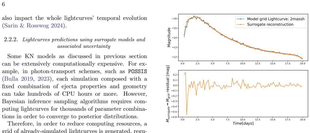
The engine of the paper is the likelihood in Eq. (1): each observed magnitude is compared with the model magnitude using a total variance $(\sigma_i^j)^2+\sigma_{\rm sys}^2$, so the single hyperparameter $\sigma_{\rm sys}$ simultaneously broadens or narrows every posterior and, at its likelihood-maximizing value, defines the model's effective goodness of fit. Two supporting metrics carry the performance analysis: the Kullback-Leibler divergence $D_{\rm KL}(P||\pi)$ between posterior and prior, computed from nested-sampling outputs, which turns information gain into a single number in nats, and the ratio of posterior to prior 68% credible intervals, which the paper shows scales roughly as $\sigma_{\rm sys}\sqrt{10/N}$. The model side is a surrogate lightcurve generator built from a grid of radiative-transfer simulations with singular-value-decomposition smoothing and Gaussian-process interpolation, whose 0.1–0.3 mag interpolation residuals are one of the contributions absorbed by $\sigma_{\rm sys}$.
What would settle it
Fit the AT2017gfo dataset with the same model and bin the residuals by time and filter: if the residual scatter grows after the first week, differs between optical and infrared bands, or correlates across filters, a single constant $\sigma_{\rm sys}$ cannot represent the model error, and the proposed goodness-of-fit metric and posterior-scaling predictions would not hold. A simpler calculation is to inject a lightcurve with known time-varying model error and check whether the likelihood-maximizing $\sigma_{\rm sys}$ still yields $\chi^2/{\rm dof}=1$ and the predicted posterior-to-prior ratios.
Extended reading notes
Core claim
On the paper's own terms, the claim is that the likelihood of Eq. (1), with a single Gaussian systematic term $\sigma_{\rm sys}$ added in quadrature to each photometric error, is the right place to absorb model imperfection, and that the $\sigma_{\rm sys}$ which maximizes the likelihood gives a principled, continuous measure of model-data compatibility. Evidence includes a toy model in which injected noise of 0.5 mag is recovered as $\sigma_{\rm sys}=0.4$ mag (with declared measurement errors of 0.3 mag), and the finding that a fixed $\sigma_{\rm sys}=1$ mag leaves AT2017gfo overfit ($\chi^2/{\rm dof}=0.26$), while freeing $\sigma_{\rm sys}$ gives about 0.57 mag. The paper further shows that posterior widths scale roughly linearly with $\sigma_{\rm sys}$, that a roughly one-per-day \textit{grizyJHK} cadence gives $D_{\rm KL}\sim8$ nats (posterior volume about 3000 times smaller than the prior), and that the information gain falls below 5–6 nats for a one-per-three-day cadence, marking the loss of ejecta constraints. Applied to AT2017gfo, the best-constrained parameter is the wind ejecta mass, and with viewing-angle and GW-distance priors the recovered masses are $\log_{10}(M_{\rm ej}^{\rm dyn}/M_\odot)=-1.92^{+0.09}_{-0.12}$ and $\log_{10}(M_{\rm ej}^{\rm wind}/M_\odot)=-1.24^{+0.09}_{-0.05}$ (95% credible intervals).
Load-bearing premise
The load-bearing premise is that all model-data discrepancies can be represented by one constant Gaussian systematic error $\sigma_{\rm sys}$ added to the measurement errors, an assumption the paper does not test for non-Gaussianity, time dependence, or correlation across filters.
Editorial extensions
If this is right
- The likelihood-maximizing $\sigma_{\rm sys}$ gives a continuous, model-to-model comparable goodness-of-fit score: a model that needs a smaller $\sigma_{\rm sys}$ is the better match to the same event.
- At a follow-up cadence of about one observation per day per filter in optical plus near-infrared bands, the joint posterior volume shrinks by roughly a factor of 3000 relative to the prior.
- A cadence of one observation every three days in each band is the practical floor for ejecta-property constraints; below it, the information gain drops below $D_{\rm KL}\sim5$–6 nats and the data mostly bound the distance.
- Combining kilonova lightcurves with independent viewing-angle and distance priors tightens ejecta-mass estimates beyond what either messenger alone provides, unless the extra priors are nearly redundant with the lightcurve information.
- Observing strategies can be optimized by filter and time window: early-time points, the $r$ band, and optical plus infrared combinations lift degeneracies most effectively.
Reading between the lines
- If $\sigma_{\rm sys}$ is adopted as a published model-comparison statistic, the natural next step is a formal model-selection test on the difference in optimal $\sigma_{\rm sys}$ between competing models, which the paper does not provide.
- The predicted cadence thresholds could be inverted into an observing-planning tool: from a target posterior compression, a telescope network could read off the minimal cadence and filter set, though this assumes the Gaussian-error model holds.
- A direct diagnostic of the constant-Gaussian assumption would be to bin the AT2017gfo fitting residuals by time and filter; correlated or late-time-growing residuals would indicate that a single $\sigma_{\rm sys}$ overstates constraints at some epochs.
Editorial analysis
A structured set of objections, weighed in public.
Referee Report
Summary. The manuscript presents a methodology-oriented study of kilonova parameter inference. It catalogues sources of uncertainty in kilonova light-curve modelling and inference, proposes the systematic-error hyperparameter sigma_sys in a Gaussian likelihood (Eq. 1) as a goodness-of-fit metric, and uses the Kullback-Leibler divergence between posterior and prior to quantify information gain. Using the Bu2019lm model in the NMMA framework, the authors simulate AT2017gfo-like light curves under different cadences, filter sets, and time windows, and report expected posterior reductions (Tables 3 and 4), a cadence threshold of roughly one observation per three days, and a comparison of simulated versus real inference performance. They then re-analyse AT2017gfo under several prior sets, report an optimal sigma_sys of about 0.57 mag, and claim final ejecta-mass estimates compatible with GW constraints from Dietrich et al. (2020).
Significance. If the proposed metric and performance forecasts were fully validated, the paper would provide practical guidance for kilonova follow-up campaigns and a simple comparative measure of model fit. The paper has clear strengths: a systematic catalogue of uncertainty sources, a substantial simulation campaign (the ManySims recovery tests), careful discussion of cadence/filter effects, and a public data release. However, the central sigma_sys metric is currently validated only under the same Gaussian assumption used to define it, and the AT2017gfo compatibility conclusions rely on priors derived from the comparison data. These issues are load-bearing for the paper's main claims, so they need to be addressed before the results can be taken at face value.
major comments (5)
- [Section 2.3, Eq. (1), Fig. 6] The validating toy model injects Gaussian noise with variance (0.5 mag)^2 and declares sigma_meas = 0.3 mag, so the recovered optimum sigma_sys = 0.4 mag is guaranteed by construction. The paper does not test the proposed goodness-of-fit metric against structured residuals, such as per-filter offsets, time-correlated errors, or outliers, which are precisely the systematic effects that sigma_sys is meant to absorb. Without a posterior predictive check or a per-filter/per-epoch residual analysis, the claim that the maximum-likelihood sigma_sys is a reasonable goodness-of-fit metric for real kilonova data is unsupported.
- [Section 3.2, Table 5] The statement that Bu2019lm 'needs' sigma_sys ~ 0.57 mag and therefore cannot fit AT2017gfo within the observational uncertainties is circular in a technical sense: sigma_sys is estimated from the same dataset to which it is then applied as a compatibility criterion. Because sigma_sys is chosen to make chi2/dof ~ 1 by construction, the quoted chi2/dof values (0.26, 0.90, 0.96, 0.97) do not constitute independent evidence of good or bad fit. A meaningful test would condition on part of the data and evaluate predictions for the remaining data, or report the full residual covariance rather than a single scalar variance.
- [Section 3.2, Table 6, prior sets C and D] The conclusion that KN-only inference with Bu2019lm gives ejecta masses compatible with GW constraints is partly built into the priors. Prior set D restricts log10 Mdyn_ej and log10 Mwind_ej to ranges derived from the Dietrich et al. (2020) GW posterior, and the resulting KN posterior is then compared with that same GW posterior. This demonstrates that the KN likelihood is not strongly inconsistent with the GW-informed region, but it cannot by itself establish compatibility or complementarity between independent messengers. The authors should either use a prior derived from data not used in the comparison, or quantify the relative evidence for prior sets C versus D in a way that does not reuse the comparison data.
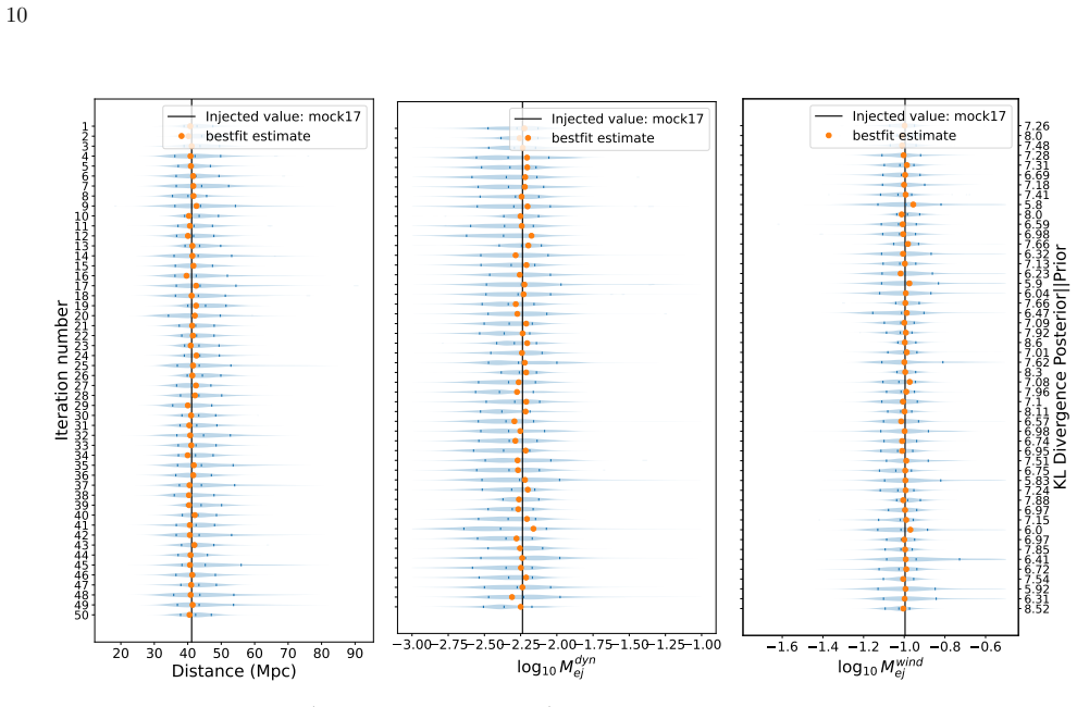
- [Section 3.1, Tables 3-4, Fig. 8] The performance forecasts (DKL ~ 8 nats, posterior volume about 3000 times smaller than the prior, and the 'one observation per three days' threshold) are conditional on a fixed Gaussian sigma_sys = 1 mag and on simulated surrogate light curves with declared 0.05 mag errors. Table 3 itself shows that posterior sizes scale by roughly a factor of two when sigma_sys changes from 1 to 0.5 mag, so the numerical forecasts cannot be quoted without an accompanying uncertainty on sigma_sys. The paper should present DKL as a function of sigma_sys, or as a distribution over it, and should soften the 'cannot constrain ejecta properties' threshold claim, which is not tied to an explicit criterion on any specific parameter.
- [Section 2.3] When sigma_sys is treated as a free parameter and sampled over, no prior on sigma_sys is specified. The reported 'maximum likelihood' value of 0.57 mag for AT2017gfo depends on whether one maximizes the profile likelihood, the posterior, or the joint likelihood; this should be stated explicitly, since the value is used throughout Section 3.2 as the basis for fixing sigma_sys = 0.6 mag.
minor comments (6)
- [Abstract and Section 3.2] There are several typos: 'sometime' should be 'sometimes' in the abstract, 'Bu2029lm' in Section 3.2 should be 'Bu2019lm', and 'toymoydel' in Appendix A.1 should be 'toymodel'.
- [Table 5] The table caption states 'Posterior 95% credible intervals' while the text in Section 3.2 sometimes reports 68% or 95% intervals without consistent notation; please clarify which intervals are shown in each part of the table and in the text.
- [Eq. (1)] The notation in Eq. (1) uses the same symbol m_j^i for both observed and model magnitudes; using e.g. m^{obs} and m^{model} would improve clarity.
- [Section 3.2, Fig. 15] The comparison of the two posterior peaks via chi2/dof values of 0.97 versus 0.96 is not a likelihood comparison; the authors should report delta log-likelihood or log-evidence if they wish to compare the peaks.
- [Figure 7] The iteration number on the y-axis is plotted as a continuous variable, which can be misleading; discrete markers or a rasterized rendering would better represent the 50 independent realizations.
- [Section 2.2.2] There is a punctuation error in 'to optimize computing cost;.'; the sentence should end with a period rather than a semicolon.
Circularity Check
No significant circularity: the sigma_sys metric is an explicit reparameterization of the reduced chi-square, and the performance forecasts are simulation-based with an external AT2017gfo consistency check.
full rationale
The derivation chain is self-contained and does not reduce to its own inputs. Eq. (1) defines the likelihood with sigma_sys added in quadrature to the observational errors, and Section 2.3 explicitly shows that, varying only sigma_sys, the likelihood is maximal when the reduced chi-square is of order unity. The proposed goodness-of-fit metric is therefore a transparent, acknowledged reparameterization of the minimized chi-square: a lower sigma_sys means smaller residuals relative to the error budget. This is not a hidden circularity because the paper presents it as a definition and recommendation, not as an independent prediction. The AT2017gfo value sigma_sys ~ 0.57 mag is obtained by maximizing the likelihood on that same dataset, and the paper does not claim to predict it from first principles; it is a fitted characterization of model-data discrepancy. The performance forecasts (DKL ~ 8 nats for 1-per-day grizyJHK, ~3.5 nats for 1-per-5-days, and the ~3000x posterior-volume reduction) are produced by simulating Bu2019lm lightcurves with fixed sigma_sys = 1 mag and a stated prior set, and the subsequent analysis of AT2017gfo with the same fixed sigma_sys is an external consistency check against real data rather than a re-use of the fitted sigma_sys. Citations to NMMA (Pang et al. 2023) and to GW-only constraints (Dietrich et al. 2020) include coauthors of the present paper, but these are public code and independent analyses used as tools or external inputs, not as authority to forbid alternatives. The unverified Gaussian and constant-sigma_sys assumption is a genuine robustness and correctness risk for the metric and for the numerical DKL values, but it is a stated modeling assumption, not a circular step.
Assumptions & free parameters
free parameters (1)
- sigma_sys (systematic error margin) =
0.57 mag (optimal for AT2017gfo); also fixed at 1.0, 0.6, 0.5, 0.2, 0 mag in analyses
assumptions (5)
- domain assumption The Bu2019lm kilonova model (Bulla 2019) with its four parameters (M_dyn, M_wind, phi, cos(iota), D_L) provides a sufficiently accurate description of kilonova emission for the performance predictions.
- domain assumption The systematic error can be modeled as a Gaussian with constant variance sigma_sys^2 added to the observational variance.
- domain assumption The surrogate model reconstructs the POSSIS grid lightcurves with RMSE < 0.3 mag for most filters (0.25 mag median).
- standard math DKL computed with Eq. 3 (mean log-likelihood minus log evidence) is an unbiased estimator of the information gain.
- standard math The likelihood (Eq. 1) factorizes over independent observations.
Cite this review
Pith. "Pith review of Kilonova modelling and parameter inference: Understanding uncertainties and evaluating compatibility between observations and models." pith.science (2026). https://pith.science/paper/45EP3KO7
@misc{pith2026250521392,
  author       = {Pith},
  title        = {Pith review of: Kilonova modelling and parameter inference: Understanding uncertainties and evaluating compatibility between observations and models},
  year         = {2026},
  howpublished = {\url{https://pith.science/paper/45EP3KO7}},
  note         = {Machine review of arXiv:2505.21392}
}
abstract
In the study of optical transients, parameter inference is the process of extracting physical information, i.e. constraints on the source's characteristics, by comparing the observed lightcurves to the predictions of different models and finding the model and parameter combination that make the closest match. In the developing field of the study of kilonovae (KNe), systematic uncertainties in modelling are still very large, and many models struggle to fit satisfactorily the whole multi-wavelength dataset of the AT2017gfo kilonova, associated to the Binary Neutron Star (BNS) merger GW170817. In a multi-messenger context, we sometime observe tensions between KN-only inference results and constraints from other messengers. In order to discuss the compatibility of KN models with observations and with the information derived from other messengers, we detail the process of Bayesian parameter inference, identifying the many sources of uncertainty embedded in KN analyses. We highlight the systematic error margin hyperparameter $\sigma_{\rm sys}$, which can be exploited as a metric for a model's goodness-of-fit. We then discuss how to assess the performance of parameter inference analyses by quantifying the information gain using the Kullback-Leibler divergence between prior and posterior. Using the example of the Bu2019lm model with the NMMA Bayesian inference framework, we showcase the expected performance that dedicated KN follow-ups with telescope networks could reasonably reach, highlighting the different factors (observational cadence, error margins) that influence such inference performances. We finally apply our KN analysis to the dataset of AT2017gfo to validate our performance predictions and discuss the complementarity of multi-messenger approaches.
Figures


Figures from the paper (12 more)




Forward citations
Cited by 2 Pith papers
-
Binary neutron stars in the next-generation era: Multi-messenger detection prospects and constraints on the equation of state, mass distribution, and cosmology
With ET (and ET+CE), mock multi-messenger BNS catalogues yield ~40–500 EM counterparts per year and, under ideal recovery, constrain R1.4 to ~0.2 km and H0 to ~1 km s−1 Mpc−1.
-
nmma: An extended Bayesian framework for Nuclear Multimessenger Astronomy in the Era of Next-Generation Detectors
nmma now jointly samples nuclear EoS parameters with GW and EM data via TOV emulators and Fiesta surrogates, delivering 20–60× speedups and future H0–nuclear constraints.
Reference graph
Works this paper leans on
-
[1]
Abbott, B. P., et al. 2017 a , Phys. Rev. Lett., 119, 161101, 10.1103/PhysRevLett.119.161101
-
[2]
---. 2017 b , Astrophys. J. Lett., 848, L13, 10.3847/2041-8213/aa920c
-
[3]
---. 2017 c , Astrophys. J. Lett., 848, L12, 10.3847/2041-8213/aa91c9
-
[4]
Anand, S., Pang, P. T. H., Bulla, M., et al. 2023, Chemical Distribution of the Dynamical Ejecta in the Neutron Star Merger GW170817. 2307.11080
arXiv 2023
-
[5]
Andrade, C., Alserkal, R., Manzano, L. S., et al. 2025, Publ. Astron. Soc. Pac., 137, 034102, 10.1088/1538-3873/adbfbc
-
[6]
Berger, E., Fong, W., & Chornock, R. 2013, Astrophys. J. Lett., 774, L23, 10.1088/2041-8205/774/2/L23
-
[7]
Blanchard, P. K., et al. 2017, Astrophys. J. Lett., 848, L22, 10.3847/2041-8213/aa9055
-
[8]
Breschi, M., Gamba, R., Carullo, G., et al. 2024, Astron. Astrophys., 689, A51, 10.1051/0004-6361/202449173
Show all 70 references
-
[9]
2021, Mon
Breschi, M., Perego, A., Bernuzzi, S., et al. 2021, Mon. Not. Roy. Astron. Soc., 505, 1661, 10.1093/mnras/stab1287
2021 doi
-
[10]
2024, Astrophys
Brethauer, D., Kasen, D., Margutti, R., & Chornock, R. 2024, Astrophys. J., 975, 213, 10.3847/1538-4357/ad7d83
2024 doi
-
[11]
2014, Astron
Buchner, J., Georgakakis, A., Nandra, K., et al. 2014, Astron. Astrophys., 564, A125, 10.1051/0004-6361/201322971
2014 doi
- [12]
- [13]
-
[14]
2018, Astrophys
Cantiello, M., et al. 2018, Astrophys. J. Lett., 854, L31, 10.3847/2041-8213/aaad64
2018 doi
-
[15]
W., Dietrich, T., Margalit, B., & Metzger, B
Coughlin, M. W., Dietrich, T., Margalit, B., & Metzger, B. D. 2019, Mon. Not. Roy. Astron. Soc., 489, L91, 10.1093/mnrasl/slz133
2019 doi
-
[16]
W., et al
Coughlin, M. W., et al. 2018, Mon. Not. Roy. Astron. Soc., 480, 3871, 10.1093/mnras/sty2174
2018 doi
-
[17]
W., Antier, S., Dietrich, T., et al
Coughlin, M. W., Antier, S., Dietrich, T., et al. 2020, Nature Communications, 11, 10.1038/s41467-020-17998-5
2020 doi
- [18]
-
[19]
J., Sneden, C., Lawler, J
Cowan, J. J., Sneden, C., Lawler, J. E., et al. 2021, Reviews of Modern Physics, 93, 10.1103/revmodphys.93.015002
2021 doi
-
[20]
2022, Mon
Curtis, S., M\"osta, P., Wu, Z., et al. 2022, Mon. Not. Roy. Astron. Soc., 518, 5313, 10.1093/mnras/stac3128
2022 doi
-
[21]
W., Pang, P
Dietrich, T., Coughlin, M. W., Pang, P. T. H., et al. 2020, Science, 370, 1450, 10.1126/science.abb4317
2020 doi
-
[22]
2017, Class
Dietrich, T., & Ujevic, M. 2017, Class. Quant. Grav., 34, 105014, 10.1088/1361-6382/aa6bb0
2017 doi
- [23]
-
[24]
J., Fryer, C
Fontes, C. J., Fryer, C. L., Hungerford, A. L., Wollaeger, R. T., & Korobkin, O. 2020, Mon. Not. Roy. Astron. Soc., 493, 4143, 10.1093/mnras/staa485
2020 doi
-
[25]
2017, Astrophys
Gao, H., Zhang, B., L\"u, H.-J., & Li, Y. 2017, Astrophys. J., 837, 50, 10.3847/1538-4357/aa5be3
2017 doi
-
[26]
2017, Astrophys
Goldstein, A., et al. 2017, Astrophys. J. Lett., 848, L14, 10.3847/2041-8213/aa8f41
2017 doi
-
[27]
W., Dietrich, T., et al
Heinzel, J., Coughlin, M. W., Dietrich, T., et al. 2021, Mon. Not. Roy. Astron. Soc., 502, 3057, 10.1093/mnras/stab221
2021 doi
-
[28]
2013, Phys
Hotokezaka, K., Kiuchi, K., Kyutoku, K., et al. 2013, Phys. Rev. D, 87, 024001, 10.1103/PhysRevD.87.024001
2013 doi
-
[29]
2019, Nature Astron., 3, 940, 10.1038/s41550-019-0820-1
Hotokezaka, K., Nakar, E., Gottlieb, O., et al. 2019, Nature Astron., 3, 940, 10.1038/s41550-019-0820-1
2019 doi
-
[30]
Jhawar, S., Wouters, T., Pang, P. T. H., et al. 2025, Phys. Rev. D, 111, 043046, 10.1103/PhysRevD.111.043046
2025 doi
-
[31]
2020, Nature Astron., 4, 77
Jin, Z.-P., Covino, S., Liao, N.-H., et al. 2020, Nature Astron., 4, 77. 1901.06269
2020 arXiv
-
[32]
2016, Nature Commun., 7, 12898, 10.1038/ncomms12898
Jin, Z.-P., Hotokezaka, K., Li, X., et al. 2016, Nature Commun., 7, 12898, 10.1038/ncomms12898
2016 doi
-
[33]
2017, Nature, 551, 80, 10.1038/nature24453
Kasen, D., Metzger, B., Barnes, J., Quataert, E., & Ramirez-Ruiz, E. 2017, Nature, 551, 80, 10.1038/nature24453
2017 doi
-
[34]
2021, Astrophys
Korobkin, O., et al. 2021, Astrophys. J., 910, 116, 10.3847/1538-4357/abe1b5
2021 doi
-
[35]
Kullback, S., & Leibler, R. A. 1951, The Annals of Mathematical Statistics, 22, 79, 10.1214/aoms/1177729694
1951
-
[36]
2024, Mon
Kunert, N., et al. 2024, Mon. Not. Roy. Astron. Soc., 527, 3900, 10.1093/mnras/stad3463
2024 doi
- [37]
-
[38]
M., & Schramm, D
Lattimer, J. M., & Schramm, D. N. 1974, Astrophys. J. Lett., 192, L145, 10.1086/181612
1974 doi
- [39]
-
[40]
1998, Astrophys
Li, L.-X., & Paczynski, B. 1998, Astrophys. J. Lett., 507, L59, 10.1086/311680
1998 doi
-
[41]
Metzger, B. D. 2017, Living Rev. Rel., 20, 3, 10.1007/s41114-017-0006-z
2017 doi
-
[42]
D., Martinez-Pinedo, G., Darbha, S., et al
Metzger, B. D., Martinez-Pinedo, G., Darbha, S., et al. 2010, Mon. Not. Roy. Astron. Soc., 406, 2650, 10.1111/j.1365-2966.2010.16864.x
2010
-
[43]
2021, Astron
Mochkovitch, R., Daigne, F., Duque, R., & Zitouni, H. 2021, Astron. Astrophys., 651, A83, 10.1051/0004-6361/202140689
2021 doi
-
[44]
P., Anderson, J., & Lu, W
Mooley, K. P., Anderson, J., & Lu, W. 2022, Nature, 610, 273, 10.1038/s41586-022-05145-7
2022 doi
-
[45]
P., Deller, A
Mooley, K. P., Deller, A. T., Gottlieb, O., et al. 2018, Nature, 561, 355, 10.1038/s41586-018-0486-3
2018 doi
-
[46]
2021, Astrophys
Nedora, V., Bernuzzi, S., Radice, D., et al. 2021, Astrophys. J., 906, 98, 10.3847/1538-4357/abc9be
2021 doi
-
[47]
2021, Mon
Nicholl, M., Margalit, B., Schmidt, P., et al. 2021, Mon. Not. Roy. Astron. Soc., 505, 3016, 10.1093/mnras/stab1523
2021 doi
-
[48]
2021, Mon
O'Connor, B., et al. 2021, Mon. Not. Roy. Astron. Soc., 502, 1279, 10.1093/mnras/stab132
2021 doi
-
[49]
2017, Astrophys
Palmese, A., et al. 2017, Astrophys. J. Lett., 849, L34, 10.3847/2041-8213/aa9660
2017 doi
-
[50]
Pang, P. T. H., et al. 2023, Nature Commun., 14, 8352, 10.1038/s41467-023-43932-6
2023 doi
-
[51]
2018 a , Astrophys
Radice, D., Perego, A., Hotokezaka, K., et al. 2018 a , Astrophys. J., 869, 130, 10.3847/1538-4357/aaf054
2018 doi
-
[52]
2018 b , Astrophys
Radice, D., Perego, A., Zappa, F., & Bernuzzi, S. 2018 b , Astrophys. J. Lett., 852, L29, 10.3847/2041-8213/aaa402
2018 doi
-
[53]
2024, Astrophys
Ragosta, F., Ahumada, T., Piranomonte, S., et al. 2024, Astrophys. J., 966, 214, 10.3847/1538-4357/ad35c1
2024 doi
-
[54]
C., Fong, W., Kilpatrick, C
Rastinejad, J. C., Fong, W., Kilpatrick, C. D., Nicholl, M., & Metzger, B. D. 2025, Astrophys. J., 979, 190, 10.3847/1538-4357/ad9c77
2025 doi
- [55]
-
[56]
2024, Astrophys
Sarin, N., & Rosswog, S. 2024, Astrophys. J. Lett., 973, L24, 10.3847/2041-8213/ad739d
2024 doi
-
[57]
F., & Finkbeiner , D
Schlafly , E. F., & Finkbeiner , D. P. 2011, , 737, 103, 10.1088/0004-637X/737/2/103
2011 doi
-
[58]
2006, Bayesian Analysis, 1, 833, 10.1214/06-BA127
Skilling, J. 2006, Bayesian Analysis, 1, 833, 10.1214/06-BA127
2006 doi
- [59]
-
[60]
2025, Astrophys
Stratta, G., et al. 2025, Astrophys. J., 979, 159, 10.3847/1538-4357/ad9b7b
2025 doi
-
[61]
2020, Mon
Tanaka, M., Kato, D., Gaigalas, G., & Kawaguchi, K. 2020, Mon. Not. Roy. Astron. Soc., 496, 1369, 10.1093/mnras/staa1576
2020 doi
-
[62]
R., Levan, A
Tanvir, N. R., Levan, A. J., Fruchter, A. S., et al. 2013, Nature, 500, 547, 10.1038/nature12505
2013 doi
-
[63]
K., Arcones , A., K \"a ppeli , R., et al
Thielemann , F. K., Arcones , A., K \"a ppeli , R., et al. 2011, Progress in Particle and Nuclear Physics, 66, 346, 10.1016/j.ppnp.2011.01.032
2011 doi
-
[64]
2018, Nature Commun., 9, 4089, 10.1038/s41467-018-06558-7
Troja, E., et al. 2018, Nature Commun., 9, 4089, 10.1038/s41467-018-06558-7
2018 doi
- [65]
-
[66]
2022, Nature, 612, 228, 10.1038/s41586-022-05327-3
---. 2022, Nature, 612, 228, 10.1038/s41586-022-05327-3
2022 doi
-
[67]
A., et al
Villar, V. A., et al. 2017, Astrophys. J. Lett., 851, L21, 10.3847/2041-8213/aa9c84
2017 doi
-
[68]
T., Fryer, C
Wollaeger, R. T., Fryer, C. L., Chase, E. A., et al. 2021, Astrophys. J., 918, 10, 10.3847/1538-4357/ac0d03
2021 doi
-
[69]
2015, Nature Commun., 6, 7323, 10.1038/ncomms8323
Yang, B., Jin, Z.-P., Li, X., et al. 2015, Nature Commun., 6, 7323, 10.1038/ncomms8323
2015 doi
-
[70]
2021, The Astrophysical Journal, 917, 24, 10.3847/1538-4357/abfe5e
Zhu, J.-P., Wu, S., Yang, Y.-P., et al. 2021, The Astrophysical Journal, 917, 24, 10.3847/1538-4357/abfe5e
2021 doi
Reviewed August 7, 2026 · model on record in the stance chip above.
Discussion (0). Sign in to comment.