REVIEW 3 major objections 5 minor 21 references
Causal Posterior Estimation
T0 review · 3 major / 5 minor · reviewed 2026-08-07 · deepseek-v4-flash
Pith's one-line read Hard-coding model structure makes posterior inference faster and sharper
desk verdict The central expressiveness claim is provably wrong for v-structures, so the benchmark results are not credible without code. read the letter →
The pith
A machine-rendered reading of the paper's core claim, the machinery that carries it, and where it could break.
The reading
What carries the argument
The load-bearing object is the structured weight matrix of the flow: a lower-triangular block matrix $B$ whose off-diagonal blocks are set to zero whenever the posterior program declares $\theta_i \perp\!\!\!\perp \theta_j \mid \theta_{\backslash ij}, x$, yielding a block neural autoregressive flow $f^{(k)}(\theta) = \mathrm{act}(B^{(k)}\theta + b^{(k)})$. Conditioning on data and time is injected by adding MLP projections of Fourier features and data to the network after the first layer, and the prior program is represented by using the prior as base distribution with a final convex combination $\gamma\theta + (1-\gamma)\lambda_t(\theta,x)$. This zero-pattern matrix is what transfers the model's causal structure into the network, so the network only models dependencies the graph says exist.
What would settle it
Estimate a posterior with CPE on a model whose naive edge-reversal posterior program is known to miss a conditional dependence (for example, a collider structure where reversing edges creates an explaining-away dependence), and test the learned posterior's conditional independence structure against the true posterior from MCMC. If the learned posterior shows a dependence where the true posterior has none (or vice versa), the zero-pattern claim fails. A second test would be to run CPE on a high-dimensional benchmark (hundreds of parameters) and compare accuracy and runtime against a transformer-based estimator; if CPE degrades more sharply, the claimed advantage does not scale.
Extended reading notes
Core claim
The central claim is that replacing a learned representation of correlations with a hard-coded representation of conditional independencies improves normalizing-flow posterior estimation. CPE sorts the parameter nodes of the posterior program in topological order and uses a block lower-triangular transformation, a block neural autoregressive flow, in which matrix blocks are zeroed exactly where $\theta_i \perp\!\!\!\perp \theta_j \mid \theta_{\backslash ij}, x$; the base distribution of the flow is the prior, and the vector field is a convex combination of identity and a learned map, motivated by exponential-family posterior mean structure. The paper reports that this architecture matches or outperforms the baselines on all nine benchmark tasks, has higher sampling acceptance rates, and that a 20-step Euler solver on a rectified flow objective performs on par with a full numerical integration solver, demonstrating constant-time $\mathcal{O}(1)$ sampling for the continuous case.
Load-bearing premise
The load-bearing premise is that zeroing flow weights according to the posterior program's conditional independencies yields a posterior with exactly those independencies, even though the base distribution is the non-factorized prior; the paper argues this by example rather than proving it.
Editorial extensions
If this is right
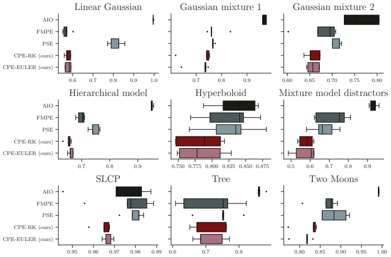
- On the nine benchmark tasks tested, CPE matches or beats FMPE, PSE, and AIO in H-min and C2ST metrics, with fewer trainable parameters when the parameter dimension is around ten.
- The 20-step Euler sampler performs on par with the Runge-Kutta 5(4) solver, showing that the rectified flow objective produces near-straight transport paths in practice.
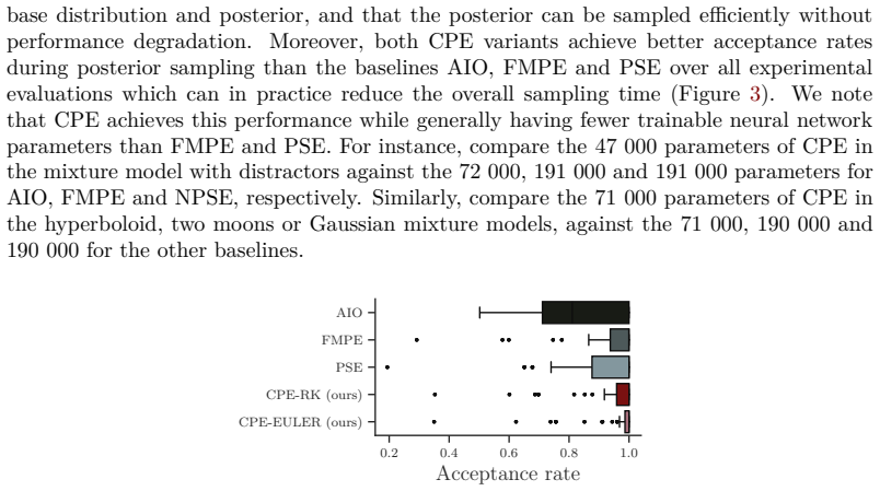
- Higher posterior-sampling acceptance rates than the baselines reduce the total number of samples needed, lowering the cost of generating posterior draws.
- Because the conditional structure is hard-coded, CPE does not need the per-layer masking or attention-based correlation refinement used by transformer posterior estimators.
- The block matrix naturally belongs to the family of structured semiseparable matrices, so future implementations could inherit sub-quadratic complexity on modern accelerators (the paper notes this is an opening, not an implemented feature).
Reading between the lines
- The reported accuracy gains are demonstrated for low-dimensional parameter spaces (on the order of ten parameters); the paper's own limitations concede the block matrix suffers from the curse of dimensionality, so whether the advantage over transformer-based methods persists at hundreds of parameters is an unverified extension.
- The method's correctness hinges on the posterior program inversion being faithful: if the naive edge reversal misses dependencies, the zero pattern is wrong and the estimator is biased rather than merely less flexible, which one could probe by comparing learned conditional-independence structure against the true posterior on models with colliders or non-reversible edges.
- If constant-time Euler sampling generalizes beyond the tested benchmarks, amortized posterior inference could become competitive with discrete flows in latency scales, enabling real-time use in simulator-based decision-making; this is a direct but untested consequence of the paper's Section 3.3 claim.
Editorial analysis
A structured set of objections, weighed in public.
Referee Report
Summary. The paper proposes Causal Posterior Estimation (CPE), an amortized simulation-based inference method that fits a normalizing flow (continuous or discrete) whose architecture is sparsified according to conditional independencies read off from a 'posterior program' obtained by reversing the edges of the generative model. The prior is used as the base distribution, the vector field is a convex combination of the identity and a learned map, and training uses a rectified-flow objective. Sampling is done with a Runge-Kutta solver or with a fixed 20-step Euler solver, advertised as O(1). Experiments on nine SBI benchmarks compare CPE against FMPE, PSE, and AIO using H-min and C2ST, reporting that CPE matches or outperforms the baselines with fewer parameters and higher acceptance rates.
Significance. If the architecture's sparsity pattern were correct, CPE would be a practically interesting way to inject model structure into neural posterior estimation. The empirical study is broad (nine benchmarks, two metrics, two training-set sizes, five seeds), and the reported strong performance, lower parameter counts, and high acceptance rates are valuable. However, the central expressiveness claim is currently unsupported and is contradicted for the paper's own motivating v-structure. The significance of the empirical results therefore depends on an unverified implementation detail: whether the experiments actually use the sparsified 'causal' architecture described in Section 3.2. The paper is transparent about the risk of naive edge reversal in Section 6, but that limitation is not peripheral; it applies to the motivating model and to several benchmarks.
major comments (3)
- [Section 3.2, Eq. (17) vs. Eq. (11)/Figure 1] For the paper's motivating model (Eq. 11, Figure 1a), the true posterior does not satisfy θ2 ⊥ θ3 | x: conditioning on the collider x induces dependence between its parents θ2 and θ3. The 'posterior program' obtained by naive edge reversal (Section 6) instead asserts θ2 ⊥ θ3 | x, and Eq. (17) accordingly zeros the coupling between θ2 and θ3 in the lower-triangular transform. Because the prior base factorizes as π(θ2)π(θ3) (θ3 is independent of θ1, θ2 a priori), the described flow factorizes as q(θ2, θ3 | x) = q(θ2 | x) q(θ3 | x) for every x. CPE therefore provably cannot represent the posterior of its own motivating example unless the implementation adds cross-variable coupling that is not documented. This is a load-bearing error, not a missing proof: the prescribed sparsity pattern encodes a conditional independence that is false.
- [Section 6 and Appendix B.7 (SLCP)] The limitation paragraph in Section 6 concedes that naively reversing edges 'may fail to capture all conditional dependencies correctly.' This is not a hypothetical concern: the SLCP benchmark (Appendix B.7) has independent parameters θ1,...,θ5 feeding a common observation x. Its true posterior does not factorize across the θi, but the reversed posterior program asserts θi ⊥ θj | x for i ≠ j, so the architecture described by Eqs. (15)-(17) is block-diagonal in θ. The competitive SLCP results in Figures 2, 5, and 6 are thus inconsistent with the architecture as described. Please state precisely, for each benchmark, which off-diagonal blocks were zeroed in the actual implementation; if no zeroing was applied, the 'hard-coding' claim needs to be substantially revised, and if zeroing was applied, the SLCP results need to be reconciled with the factorization argument above.
- [Sections 3.1-3.2 (base distribution and zero pattern)] The claim that a lower-triangular flow with zeros matching a posterior-program conditional independence is sufficiently expressive to represent the posterior is asserted ('we argue') and never proved. It is also generally false when the prior base is not factorized in the same way: a block-diagonal transform θi' = fi(θi; x), θj' = fj(θj; x) maps the base density to q(θi, θj | x) = π(θi, θj) / |det J|, which factorizes only if π(θi, θj) does. Since CPE uses the (generally non-factorized) prior as base (Eq. 13 and Section 3.1), the flow cannot enforce a posterior conditional independence that is absent from the prior. The expressiveness argument needs a proof or a concrete construction; otherwise the central claim of the paper is unsupported.
minor comments (5)
- [Abstract and Section 3.3] A fixed 20-step Euler solver takes a constant number of steps, but the per-step cost grows with the parameter dimension and network width, so 'constant-time O(1)' is not an accurate complexity statement; please say 'fixed number of steps' or 'constant number of neural network evaluations' instead.
- [Equations (7) and (26)] The displayed formula for the optimal-transport vector field appears garbled: the numerator and denominator contain θ where θ(1) and t are intended. Please correct these equations and check the derivation, since they affect the reproducibility of the FMPE baseline.
- [Section 3.4] The word 'bifurcation' in the description of finding the inverse of the discrete flow should presumably be 'bisection' (or 'root finding via bisection').
- [Appendix C.1] The sentence 'the reference posterior sample consists of 50 00particles' contains a typo and the sample-size accounting is unclear: ten chains, 10,000 draws, 5,000 warmup, thinning every second would yield a different number; please clarify.
- [Figures 2 and 5-8] With five seeds per condition, the figures would benefit from error bars or at least a statement that they are omitted; as presented, the reader cannot assess variability across seeds.
Circularity Check
No significant circularity: CPE's posterior approximation is learned from simulated data and evaluated against held-out benchmarks; the flagged caveats are correctness risks, not input-output equivalences.
full rationale
The paper's central claim is that hard-coding the conditional dependence structure of the prior and posterior programs into a normalizing-flow architecture yields accurate amortized posterior inference. No step in the derivation reduces a prediction to its input by construction. The architecture is trained with a flow-matching/rectified-flow objective on synthetic (θ, x) pairs from the simulator, and accuracy is measured against MCMC reference posteriors on held-out benchmark observations. The use of the prior as the base distribution (Section 3.1) and the convex combination in Eq. 13 are modeling choices, not fitted constants that preordain the reported posterior quality. The sparsity pattern in Section 3.2 is derived from the graphical model, but the resulting flow is still trained to match the true posterior through the simulation-based objective; it is not defined to equal that posterior. The self-citations to the authors' sbijax package and to their own H-min divergence are implementation and evaluation-tool choices; they do not constitute load-bearing mathematical premises that force the outcome. The v-structure concern raised by the skeptic is a genuine correctness/expressiveness issue: naively reversing edges (Section 6) may encode a conditional independence that the true posterior lacks, making the architecture biased on such models. That is a false-assumption risk, explicitly acknowledged as a limitation by the authors, not a circular step in which the claimed prediction is equivalent to an input. Overall, the paper's derivation chain is self-contained and independently testable.
Assumptions & free parameters
free parameters (3)
- gamma (convex-combination gate) =
trainable, not reported
- Euler steps T =
20
- Architecture hyperparameters =
K=3, block size 64, Fourier features 64, MLP widths 64 and 128
assumptions (4)
- domain assumption The posterior program is a DAG and can be topologically ordered.
- ad hoc to paper A lower-triangular flow with zeros matching posterior conditional independencies is sufficiently expressive to represent the posterior.
- ad hoc to paper Naively reversing the edges of the generative model gives the correct posterior conditional independence structure.
- domain assumption Rectified-flow training yields sufficiently straight trajectories that 20 Euler steps sample accurately.
Cite this review
Pith. "Pith review of Causal Posterior Estimation." pith.science (2026). https://pith.science/paper/K64XJXM2
@misc{pith2026250521468,
  author       = {Pith},
  title        = {Pith review of: Causal Posterior Estimation},
  year         = {2026},
  howpublished = {\url{https://pith.science/paper/K64XJXM2}},
  note         = {Machine review of arXiv:2505.21468}
}
read the original abstract
We present Causal Posterior Estimation (CPE), a novel method for Bayesian inference in simulator models, i.e., models where the evaluation of the likelihood function is intractable or too computationally expensive, but where one can simulate model outputs given parameter values. CPE utilizes a normalizing flow-based (NF) approximation to the posterior distribution which carefully incorporates the conditional dependence structure induced by the graphical representation of the model into the neural network. Thereby it is possible to improve the accuracy of the approximation. We introduce both discrete and continuous NF architectures for CPE and propose a constant-time sampling procedure for the continuous case which reduces the computational complexity of drawing samples to O(1) as for discrete NFs. We show, through an extensive experimental evaluation, that by incorporating the conditional dependencies induced by the graphical model directly into the neural network, rather than learning them from data, CPE is able to conduct highly accurate posterior inference either outperforming or matching the state of the art in the field.
Figures


Figures from the paper (5 more)



Reference graph
Works this paper leans on
-
[1]
Albergo, M. S., & Vanden-Eijnden, E. (2023). Building normalizing flows with stochastic interpolants. The Eleventh International Conference on Learning Representations. Albert, C., Künsch, H. R., & Scheidegger, A. (2015). A simulated annealing approach to approximate Bayes computations.Statistics and Computing, 25, 1217–1232. Albert, C., Ulzega, S., Ozdem...
work page 2023
-
[2]
I is a ten-dimensional vector of ones
= abs ( ||θ−x1||2−||θ−x2||2 ) , and scale matrixσ2I. I is a ten-dimensional vector of ones. We follow Forbes et al. (2022) and set a1 = [−0.5, 0.0]T, a2 = [0.5, 0.0]T, b1 = [0.0,−0.5]T, b2 = [0.0, 0.5]T, ν = 3 and σ2 = 0.01 for our experiments. B.6 Mixture model with distractors Similarly to the SLCP task (Lueckmann et al., 2021), we evaluate a benchmark ...
work page 2022
-
[3]
23 B.8 Tree The tree model is a recently introduced SBI benchmark model (Gloeckler et al., 2024)
fori = 1,..., 5 µ(θ) = (θ1,θ 2),ϕ 1 =θ2 3,ϕ 2 =θ2 4 Σ(θ) = ( ϕ2 1 tanh(θ5)ϕ1ϕ2 tanh(θ5)ϕ1ϕ2 ϕ2 2 ) xj|θ∼N (xj;µ(θ), Σ(θ)) forj = 1,..., 4 x = [x1,...,x 4]T Henceθ∈ R5 is a five-dimensional random variable, while the datax has eight dimensions. 23 B.8 Tree The tree model is a recently introduced SBI benchmark model (Gloeckler et al., 2024). It has the foll...
work page 2024
-
[10]
The GMM follows the representation in Lueckmann et al
x|θ∼ 1 2N2(θ,I ) + 1 2N2(θ,σ 2I) where σ2 = 0.01, I is a unit matrix, and bothθ∈ R2 and x∈ R2 are two-dimensional random variables. The GMM follows the representation in Lueckmann et al. (2021). B.3 Gaussian mixture 2 The Gaussian mixture 2 has been proposed in Vargas et al. (2024). It is a 3-component mixture that we adapted for SBI. It has the following...
work page 2021
-
[14]
simple likelihood complex posterior
where we set α = σ = 0.3. In addition to the two informative data dimensions x1,x 2, the model adds 8 samples from a standard Gaussian that do not carry information of the parameters. If both x1,obs and x2,obs are from the same mode (in our experiments we set x1,obs =x2,obs = 5), then the posterior forθ is bimodal with very uneven mass distribution. B.7 S...
work page 2019
-
[16]
Its generative process is defined as: θ∼U 2(−10,
x1∼N ( sin(θ2)2, 0.22 ) x2∼N ( θ2 2, 0.22 ) x2∼N ( 0.1θ2 3, 0.62 ) x3∼N ( cos(θ3)2, 0.12 ) B.9 Two moons Two moons is a common benchmark task in the SBI literature (Greenberg et al., 2019). Its generative process is defined as: θ∼U 2(−10,
work page 2019
-
[18]
can be computed via the chain rule: log ⏐⏐⏐⏐det∂f ∂θ ⏐⏐⏐⏐= dθ∑ i=1 log (∂f ∂θ ) ii = dθ∑ i=1 log ( ∂f (K) ∂f (K−1) ∂f (K−1) ∂f (K−2) ... ∂f (1) ∂θ ) ii = dθ∑ i=1 logg(B(K) ii )⋆ log ∂act h (K−2) i ⋆··· ⋆ logg(B(1) ii ) where Bii are matrices (see Section 3.2) andh(K−2) i the diagonal elements of the output of function f(K−2) which depend onθi, and where w...
work page 2019
-
[19]
To faihfully compare AIO against CPE, we use directed graphs as masks for AIO. 25 FMPE FMPE uses a two-layer MLP with 128 nodes each to embed parameter valuesθ and a two-layer MLP with 128 nodes each to embed data valuesx. We first project time valuest through random Fourier features of dimensionality64, before embedding the result using a two-layer MLP w...
work page 2023
Show all 21 references
-
[20]
C.4 Training Each neural SBI method (i.e., CPE and all baselines) are trained using an Adam optimizer (Kingma & Ba,
All activation functions are SiLUs (Hendrycks & Gimpel, 2016). C.4 Training Each neural SBI method (i.e., CPE and all baselines) are trained using an Adam optimizer (Kingma & Ba,
2016
-
[23]
discrete
Lipman et al. (2023) define a particularly useful parameterization for the conditional density path based on Gaussian transition kernels and the respective conditional vector field: ϱt(θ|θ(1)) =N (tθ(1), (1− (1−σmin)t)2I) ut(θ|θ(1)) = θ1− (1−σmin)θ 1− (1−σmin)θ (26) where σmin...
2023
-
[29]
Papamakarios, G., Pavlakou, T., & Murray, I. (2017). Masked autoregressive flow for density estimation. Advances in Neural Information Processing Systems. Papamakarios, G., Sterratt, D., & Murray, I. (2019). Sequential neural likelihood: Fast likelihood-free inference with aut...
2017 arXiv
-
[30]
Vehtari, A., Gelman, A., Simpson, D., Carpenter, B., & Bürkner, P.-C. (2021). Rank- normalization, folding, and localization: An improvedˆR for assessing convergence of MCMC.Bayesian analysis, 16(2), 667–718. Verma, Y., Bharti, A., & Garg, V. (2025). Robust simulation-based in...
2021 arXiv
-
[34]
De Cao, N., Aziz, W., & Titov, I. (2020). Block neural autoregressive flow.Proceedings of The 35th Uncertainty in Artificial Intelligence Conference. Deistler, M., Goncalves, P. J., & Macke, J. H. (2022). Truncated proposals for scalable and hassle-free simulation-based infere...
2020 arXiv
-
[43]
Ambrogioni, L., Silvestri, G., & van Gerven, M. (2021). Automatic variational inference with cascading flows.Proceedings of the 38th International Conference on Machine Learning. Babuschkin, I., Baumli et al. (2020).The DeepMind JAX Ecosystem. Beaumont, M. A., Cornuet, J.-M., ...
2021
-
[85]
T., Robert, C
Frazier, D. T., Robert, C. P., & Rousseau, J. (2020). Model misspecification in approxi- mate Bayesian computation: Consequences and diagnostics.Journal of the Royal Statistical Society Series B: Statistical Methodology, 82(2), 421–444. Fu, D. Y., Arora, S., Grogan, J., Johnso...
2020
-
[1143]
Lipman, Y., Chen, R. T. Q., Ben-Hamu, H., Nickel, M., & Le, M. (2023). Flow match- ing for generative modeling. The Eleventh International Conference on Learning Representations. 14 Liu, X., Gong, C., & qiang liu. (2023). Flow straight and fast: Learning to generate and transf...
2023
-
[2015]
We trained each method to convergence with a maximum of2 000 training epochs (whichever is fulfilled first)
with learning ratelr = 0.0001 and β1 = 0.9 and β2 = 0.999. We trained each method to convergence with a maximum of2 000 training epochs (whichever is fulfilled first). We used10% of the simulated data as a validation set. We useOptax for gradient-based optimization (Babuschkin...
2020
-
[2021]
and effective sample size as implemented in the Python package Kumar et al. (2019). 24 C.2 Comparing reference posteriors to inferred posteriors We compare the inferred posterior distributions to the reference posterior distributions us- ing the classifier-two-sample-test stat...
2019
-
[2022]
To compute the metrics, we first subsample both reference and inferred posteriors to10 000 samples, and then compute both metrics
which we, like Dirmeier, Albert, and Perez-Cruz (2023), found to be easier to tune than C2ST and other divergences. To compute the metrics, we first subsample both reference and inferred posteriors to10 000 samples, and then compute both metrics. C.3 Neural network architectur...
2023
-
[2024]
We describe the different models below
and develop new benchmark tasks. We describe the different models below. B.1 Linear Gaussian The linear Gaussian benchmark task is defined by the following generative process: θ∼N 10(0,σ 2I) (31) x|θ∼N 10(θ,σ 2I) (32) whereσ2 = 0.1,I is a unit matrix of appropriate dimensional...
2021
-
[2025]
Geffner, T., & Domke, J. (2023). Langevin diffusion variational inference.Proceedings of The 26th International Conference on Artificial Intelligence and Statistics. Geffner,T.,Papamakarios,G.,&Mnih,A.(2023).Compositionalscoremodelingforsimulation- based inference.Internationa...
2023 arXiv
Reviewed August 7, 2026 · model on record in the stance chip above.
Discussion (0). Sign in to comment.