REVIEW 2 major objections 5 minor 1 cited by
The ESPRESSO Redshift Drift Experiment I -- High-resolution spectra of the Lyman-$\alpha$ forest of QSO J052915.80-435152.0
T0 review · 2 major / 5 minor · reviewed 2026-08-07 · deepseek-v4-flash
Pith's one-line read A two-epoch Lyman-\alpha forest measurement of the brightest known quasar yields a velocity drift consistent with zero, at a precision only about 10 percent above the photon-noise prediction.
desk verdict A solid first step on the ESPRESSO redshift-drift program that hits the expected precision, but the model-based estimator's claimed unbiasedness rests on an untested cancellation. read the letter →
The pith
A machine-rendered reading of the paper's core claim, the machinery that carries it, and where it could break.
The reading
What carries the argument
The load-bearing object is the model-based differential shift estimator. An ensemble of 500 cubic-spline models of the combined quasar spectrum is generated with an inter-knot spacing of about $8.4\ {\rm km\,s^{-1}}$, a spacing calibrated so that residuals on mock spectra drawn from hydrodynamical simulations follow a standard normal distribution. For each epoch, a Markov-chain Monte Carlo scan evaluates a modified Gaussian likelihood in which the spline nodes are rigidly shifted by $\delta v$, pixel noise and model variance are added in quadrature, and pixels are weighted by the mean spectral gradient divided by the model-scatter of that gradient, so steep, well-constrained line edges dominate. The reported drift is the difference $\Delta v = \delta v_2 - \delta v_1$; this subtraction is the step that converts two epoch measurements into the cosmological quantity.
What would settle it
Generate many mock epoch pairs with zero true drift, matching the signal-to-noise, masking, and weighting scheme used here, and run the model-based pipeline on each pair; if the recovered $\Delta v$ distribution is not centred on zero within the quoted uncertainties, the null result is biased. The paper's own combined-spectrum null test provides the template for this check.
Extended reading notes
Core claim
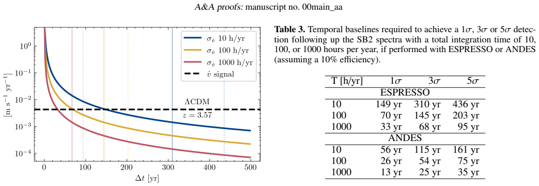
The paper's central result is a null measurement of the Sandage signal: between the two epochs the Lyman-$\alpha$ forest of the quasar shifts by $\Delta v = -1.25^{+4.44}_{-4.46}\ {\rm m\,s^{-1}}$, equivalent to $\dot{z} = (-2.19^{+7.75}_{-7.78})\times 10^{-8}\ {\rm yr^{-1}}$, fully consistent with zero and with $\Lambda$CDM. The durable claim is that the model-based method reaches a statistical uncertainty only about 10 percent above the photon-noise precision predicted by the standard scaling relation, even though this is a single sightline subject to cosmic variance. Systematic checks reported in the paper find that local Solar-system acceleration, wavelength-calibration differences, and the quasar's proximity region each contribute less than the statistical error at the current signal-to-noise. The paper extrapolates from this performance that a $3\sigma$ detection of the cosmic drift would require roughly 145 years of ESPRESSO monitoring or 54 years with an ELT-class spectrograph at 100 hours per year.
Load-bearing premise
The result assumes the model-based estimator measures the true velocity difference between the two epochs without bias, even though the same estimator returns about $-2.7 \pm 2.1\ {\rm m\,s^{-1}}$ when the combined spectrum is measured against its own model ensemble with the chosen weighting, and about $-0.4 \pm 3.5\ {\rm m\,s^{-1}}$ without it; whether that weighting bias cancels in the difference is not demonstrated.
Editorial extensions
If this is right
- The measured $\Delta v = -1.25 \pm 4.45\ {\rm m\,s^{-1}}$ places a new direct limit on cosmic acceleration from a Lyman-$\alpha$ sightline, about 2.3 times looser than the best previous limit from HI 21 cm absorbers, but obtained with 12.4 hours of data instead of a 13-year baseline.
- If the single-sightline precision holds, the exposure-time scaling for the planned ELT/ANDES experiment is empirically anchored: a $3\sigma$ detection needs roughly 5400 hours over 54 years at 100 hours per year and 10 percent efficiency.
- The spline-ensemble estimator outperforms the pixel-by-pixel method by about 30 percent on this dataset, establishing the model-based pipeline as the route for combining future epochs.
- At the current precision, Solar-system acceleration, wavelength-calibration method differences, and the exclusion of the quasar proximity region each shift the result by less than the statistical uncertainty, so no large correction is yet required.
- Combining the two epochs into a single baseline measurement demonstrates that the Lyman-$\alpha$ forest of one exceptionally bright quasar can already deliver the velocity precision needed to plan a decades-long cosmological monitoring programme.
Reading between the lines
- The paper leaves open whether the weighting-induced bias seen in its combined-spectrum null test, about $-2.7\ {\rm m\,s^{-1}}$ with the chosen weights versus $-0.4\ {\rm m\,s^{-1}}$ with uniform weights, cancels in the difference; this is testable by running the same pipeline on mock epoch pairs with zero true drift.
- The 54-year projection for the ELT assumes this target's performance transfers to other quasars; sightline-to-sightline cosmic variance in the number and width of Lyman-$\alpha$ lines could shorten or lengthen that timeline, a question the parallel analysis of the second brightest target should answer.
- The same calibrated-spline-ensemble estimator, with its explicit model-variance term, could be adapted to other high-precision spectroscopic shift measurements, such as searches for variation of fundamental constants, provided the null-weighting bias is characterized first.
Editorial analysis
A structured set of objections, weighed in public.
Referee Report
Summary. The paper reports the first two-epoch ESPRESSO redshift-drift experiment on the Lyman-alpha forest of the bright quasar J052915.80-435152.0 (SB2). After masking metal lines and a sub-DLA, the authors apply a Bouchy et al. pixel-by-pixel method and a newly developed spline-based model method calibrated on Sherwood mock spectra. The model-based method yields Δv = -1.25 +4.44/-4.46 m/s between epochs separated by 0.875 yr, equivalent to zdot = (-2.19 +7.75/-7.78) x 10^-8 /yr, consistent with zero and with the Lambda-CDM expectation. The model-based uncertainty is about 10% above the Liske et al. precision prediction. The paper also extrapolates to an ELT/ANDES campaign, estimating 5400 hours over 54 years for a 3-sigma detection.
Significance. If the measurement is unbiased, this is an important step: it demonstrates that a single bright ESPRESSO sightline can reach the predicted precision for the Lyman-alpha forest redshift-drift experiment, validates an analysis pipeline for ANDES, and provides the first empirical anchor for planning the ELT monitoring campaign. The paper is commendably transparent about the W-weighting null-test offset and includes mock-based validation, spectral-chunk stability checks, and calibration systematics tests. The main unresolved issue is whether the W-induced bias cancels in the epoch difference, which is the quantity of scientific interest.
major comments (2)
- [Sec. 6.4 (Eqs. 11-12)] The weighted likelihood null test gives δv0 = -2.71 ± 2.08 m/s on the combined spectrum against its own model ensemble, whereas fixing W=1 gives -0.43 ± 3.51 m/s. The paper interprets δv0 as falling between δv1 and δv2 and therefore concludes that the negative δv1 and δv2 are not surprising. This is not a demonstration that the W-induced bias cancels in Δv = δv2 - δv1, which is the scientific quantity. Because the model is built from the combined spectrum and the two epochs have different median S/N (47 for epoch 1, 72 for epoch 2), the bias for the two epoch fits need not be identical. A differential bias of order 1-2 m/s would shift the central value by an amount that is not negligible relative to the reported statistical uncertainty and would become increasingly important as the S/N grows. The authors should quantify this directly: report Δv, δv1, and δv2 for W=1; perform injection-recovery tests on the real spectra with injected shifts of order ±1 to ±5 m/s; and/or estimate the bias as a function of S/N. Without this, the central null value has an unquantified systematic component.
- [Sec. 7.1 and Fig. 7] The mock-injection validation is not decisive for the W-weighting bias. Only 10 sightlines are used per injected shift, and at the 0.875-yr baseline the injected shift is -0.38 cm/s, more than two orders of magnitude smaller than the -2.71 m/s null-test offset reported in Sec. 6.4. The zero-drift mock set is the relevant control, but the paper does not report the mean and scatter of the model-based Δv for that case; with 10 sightlines and per-sightline uncertainties of order 4 m/s, the standard error of the mean would be about 1.3 m/s, so a -2.7 m/s bias would be marginally detectable. Reporting these numbers, and ideally bias as a function of S/N, would directly test whether the bias cancels in Δv = δv2 - δv1.
minor comments (5)
- [Sec. 7.5] The LSF systematic uncertainty is estimated by analogy with the LFC/FP difference rather than measured directly; this should be stated as a rough estimate and propagated as a systematic in future epochs.
- [Table 2] The absorption system at z=3.29 appears twice in the table; please verify whether one entry is spurious.
- [Table 1] The start time of the 2023-02-22 exposure is written as '00:54.53' instead of '00:54:53'.
- [Sec. 7.3] The 5.14 m/s shift upon excluding the proximity region is attributed to the reduced pixel sample and S/N, but the explanation is qualitative; consider adding this as a systematic term or providing a quantitative test.
- [Sec. 4, Eq. 5] Equation 5 is described as an adaptation of Liske et al., but the derivation of the form factor and the f_Lyα dependence is not given; a brief derivation or reference would help reproducibility.
Circularity Check
No significant circularity: the reported drift is a differential measurement whose model anchor cancels, and all calibrating inputs are external or statistically independent.
full rationale
The central quantity Delta v = delta v2 - delta v1 is not fitted to itself. The spline model is built from the combined spectrum, but the model acts only as a common reference: to first order, any model bias common to the two epoch fits cancels in the difference, and the paper explicitly verifies recovery of known injected shifts on mock spectra (Fig. 7). The mock data are used solely to calibrate the spline knot spacing A and to validate the pipeline; the authors state 'We stress that the mock data were only used to calibrate the modelling procedure and are not involved in the final measurement.' The null-test offset delta v0 = -2.71 m/s with the W weighting, and -0.43 m/s with W=1, is an acknowledged systematic property of the weighting scheme, not a hidden input to Delta v; the final result is the difference of two separately measured shifts, and the paper does not claim delta v0 as a prediction. The precision comparison uses the external Liske et al. (2008) scaling relation as a benchmark. Self-citations (e.g., Cristiani et al. 2024 for metal-line dynamics, Trost et al. 2025 for the noise prescription) are independent published studies with their own data and do not constitute a load-bearing circular chain. The residual concern that the W-induced bias might not cancel exactly in Delta v is a systematic-uncertainty/validation question, not a circularity of derivation, and is appropriately left as a caveat for the differential measurement.
Assumptions & free parameters
free parameters (3)
- Spline internodal distance A =
8.37 (+0.26, -0.24) km/s
- ANDES total efficiency epsilon =
0.1 (assumed)
- Monitoring cadence T =
100 h/yr in the baseline projection
assumptions (5)
- domain assumption Lyman-alpha forest absorbers trace the Hubble flow with negligible peculiar accelerations, so a rigid velocity shift between epochs is the cosmological signal.
- ad hoc to paper The optimal spline knot spacing A calibrated on Sherwood mocks transfers to the real SB2 spectrum.
- ad hoc to paper The W weighting in Eq. 11 does not bias the differential shift Delta v = delta v_2 - delta v_1.
- domain assumption ESPRESSO wavelength calibration and line-spread function are stable between P110 and P112.
- domain assumption The Liske et al. precision scaling relation applies to a single bright sightline.
Cite this review
Pith. "Pith review of The ESPRESSO Redshift Drift Experiment I -- High-resolution spectra of the Lyman-$\alpha$ forest of QSO J052915.80-435152.0." pith.science (2026). https://pith.science/paper/LKTAODJW
@misc{pith2026250521615,
  author       = {Pith},
  title        = {Pith review of: The ESPRESSO Redshift Drift Experiment I -- High-resolution spectra of the Lyman-$\alpha$ forest of QSO J052915.80-435152.0},
  year         = {2026},
  howpublished = {\url{https://pith.science/paper/LKTAODJW}},
  note         = {Machine review of arXiv:2505.21615}
}
abstract
The measurement of the temporal evolution in the redshift of distant objects, the redshift drift, is a probe of universal expansion and cosmology. We perform the first steps towards a measurement of such effect using the Lyman-$\alpha$ forest in the spectra of bright quasars as a tracer of cosmological expansion. Our goal is to determine to which precision a velocity shift measurement can be carried out with the signal-to-noise (S/N) level currently available and whether this precision aligns with previous theoretical expectations. A precise assessment of the achievable measurement precision is fundamental for estimating the time required to carry out the whole project. We acquire 12 hours of ESPRESSO observations distributed over 0.875 years of the brightest quasar known, J052915.80-435152.0 (z=3.962), to obtain high-resolution spectra of the Lyman-$\alpha$ forest, with median S/N of ~86 per 1 km/s pixel at the continuum. We divide the observations into two epochs and analyse them using both a pixel-by-pixel method and a model-based approach. This comparison allows us to estimate the velocity shift between the epochs, as well as the velocity precision that can be achieved at this S/N. The model-based method is calibrated using high-resolution simulations of the intergalactic medium, and it provides greater accuracy compared to the pixel-by-pixel approach. We measure a velocity drift of the Lyman-$\alpha$ forest consistent with zero: $\Delta v = -1.25\pm 4.45 {\rm ms^{-1}}$, equivalent to a cosmological drift of $\dot{v}=-1.43\pm 5.09 {\rm ms^{-1}yr^{-1}}$ or $\dot{z}= (-2.19\pm7.77) \times 10^{-8}{\rm yr^{-1}}$. The measurement uncertainties are on par with the expected precision. We estimate that reaching a 99% detection of the cosmic drift requires a monitoring campaign of 5400 hours of integration time over 54 years with an ELT and an ANDES-like high-resolution spectrograph.
Figures


Figures from the paper (6 more)


Forward citations
Cited by 1 Pith paper
-
Nonlinear Relativistic Effects on Cosmological Redshift Drift
Second-order relativistic effects on redshift drift are computed, showing distortions appear only at this order with enhanced nonlinear bispectrum contributions at low redshift and large momenta.
Reference graph
Works this paper leans on
-
[1]
G., Aguilar, J., Ahlen, S., et al
Adame, A. G., Aguilar, J., Ahlen, S., et al. 2025, J. Cosmology Astropart. Phys., 2025, 021
2025
-
[2]
2006, arXiv e-prints, astro
Albrecht, A., Bernstein, G., Cahn, R., et al. 2006, arXiv e-prints, astro
2006
-
[3]
Alves, C. S., Leite, A. C. O., Martins, C. J. A. P., Matos, J. G. B., & Silva, T. A. 2019, Mon. Not. Roy. Astron. Soc., 488, 3607
work page 2019
-
[4]
Becker, G. D. & Bolton, J. S. 2013, MNRAS, 436, 1023
work page 2013
-
[5]
Bolton, A. S. & Schlegel, D. J. 2010, PASP, 122, 248
work page 2010
-
[6]
S., Puchwein, E., Sijacki, D., et al
Bolton, J. S., Puchwein, E., Sijacki, D., et al. 2017, MNRAS, 464, 897
work page 2017
-
[7]
2001, A&A, 374, 733
Bouchy, F., Pepe, F., & Queloz, D. 2001, A&A, 374, 733
2001
-
[8]
Calderone, G., Boutsia, K., Cristiani, S., et al. 2019, ApJ, 887, 268
work page 2019
Show all 48 references
-
[9]
2020, MNRAS, 492, 2044
Cooke, R. 2020, MNRAS, 492, 2044
2020
-
[10]
2024, MNRAS, 528, 6845
Cristiani, S., Cupani, G., Trost, A., et al. 2024, MNRAS, 528, 6845
2024
-
[11]
2023, MNRAS, 522, 2019
Cristiani, S., Porru, M., Guarneri, F., et al. 2023, MNRAS, 522, 2019
2023
-
[12]
2016, in Society of Photo-Optical Instrumentation Engineers (SPIE) Conference Series, V ol
Cupani, G., D’Odorico, V ., Cristiani, S., et al. 2016, in Society of Photo-Optical Instrumentation Engineers (SPIE) Conference Series, V ol. 9913, Software and Cyberinfrastructure for Astronomy IV , ed. G. Chiozzi & J. C. Guzman, 99131T
2016
-
[13]
2020, in Software and Cyber- infrastructure for Astronomy VI, ed
Cupani, G., D’Odorico, V ., Cristiani, S., et al. 2020, in Software and Cyber- infrastructure for Astronomy VI, ed. J. C. Guzman & J. Ibsen, V ol. 11452, International Society for Optics and Photonics (SPIE), 372 – 388
2020
-
[14]
2012, Astrophys
Darling, J. 2012, Astrophys. J., 761, L26
2012
-
[15]
S., Kneib, J.-P., Percival, W
Dawson, K. S., Kneib, J.-P., Percival, W. J., et al. 2016, AJ, 151, 44
2016
-
[16]
S., Schlegel, D
Dawson, K. S., Schlegel, D. J., Ahn, C. P., et al. 2013, AJ, 145, 10 Di Marcantonio, P., Sosnowska, D., Cupani, G., et al. 2018, in Society of Photo- Optical Instrumentation Engineers (SPIE) Conference Series, V ol. 10704, Ob- servatory Operations: Strategies, Processes, and S...
2013
-
[17]
2014, arXiv e-prints, arXiv:1405.0484 Gaia Collaboration, Brown, A
Fienga, A., Manche, H., Laskar, J., Gastineau, M., & Verma, A. 2014, arXiv e-prints, arXiv:1405.0484 Gaia Collaboration, Brown, A. G. A., Vallenari, A., et al. 2021, A&A, 649, A1
2014 arXiv
-
[18]
M., Kirshner, R
Garnavich, P. M., Kirshner, R. P., Challis, P., et al. 1998, ApJ, 493, L53
1998
-
[19]
2021, Phys
Heinesen, A. 2021, Phys. Rev. D, 103, L081302
2021
-
[20]
2020, PASJ, 72, L1
Inoue, T., Komatsu, E., Aoki, W., et al. 2020, PASJ, 72, L1
2020
-
[21]
2025, ApJ, 982, 177
Kang, J., Zhang, T.-J., He, P., & Zhu, M. 2025, ApJ, 982, 177
2025
-
[22]
S., Carswell, R
Kim, T. S., Carswell, R. F., Cristiani, S., D’Odorico, S., & Giallongo, E. 2002, MNRAS, 335, 555 Klöckner, H.-R., Obreschkow, D., Martins, C., et al. 2015, PoS, AASKA14, 027
2002
-
[23]
K., Milakovi ´c, D., & Carswell, R
Lee, C.-C., Webb, J. K., Milakovi ´c, D., & Carswell, R. F. 2021, MNRAS, 507, 27
2021
-
[24]
2008, MNRAS, 386, 1192 Lo Curto, G., Pepe, F., Avila, G., et al
Liske, J., Grazian, A., Vanzella, E., et al. 2008, MNRAS, 386, 1192 Lo Curto, G., Pepe, F., Avila, G., et al. 2015, The Messenger, 162, 9
2008
-
[25]
2024, in Society of Photo-Optical Instrumentation Engineers (SPIE) Conference Series, V ol
Marconi, A., Abreu, M., Adibekyan, V ., et al. 2024, in Society of Photo-Optical Instrumentation Engineers (SPIE) Conference Series, V ol. 13096, Ground- based and Airborne Instrumentation for Astronomy X, ed. J. J. Bryant, K. Mo- tohara, & J. R. D. Vernet, 1309613
2024
-
[26]
Marques, C. M. J., Martins, C. J. A. P., & Alves, C. S. 2023, MNRAS, 522, 5973
2023
-
[27]
Marques, C. M. J., Martins, C. J. A. P., & Gilabert López, B. 2024, MNRAS, 527, 9918
2024
-
[28]
Martins, C. J. A. P. et al. 2024, Exper. Astron., 57, 5
2024
-
[29]
McVittie, G. C. 1962, ApJ, 136, 334 Milakovi´c, D., Webb, J. K., Molaro, P., et al. 2024, MNRAS, 534, 12
1962
-
[30]
2014, A&A, 567, A25
Noll, S., Kausch, W., Kimeswenger, S., et al. 2014, A&A, 567, A25
2014
-
[31]
A., Wolf, C., Bessell, M
Onken, C. A., Wolf, C., Bessell, M. S., et al. 2024, PASA, 41, e061
2024
-
[32]
2021, A&A, 645, A96 Péroux, C., McMahon, R
Pepe, F., Cristiani, S., Rebolo, R., et al. 2021, A&A, 645, A96 Péroux, C., McMahon, R. G., Storrie-Lombardi, L. J., & Irwin, M. J. 2003, MN- RAS, 346, 1103
2021
-
[33]
2021, A&A, 646, A32 Planck Collaboration, Aghanim, N., Akrami, Y ., et al
Piskunov, N., Wehrhahn, A., & Marquart, T. 2021, A&A, 646, A32 Planck Collaboration, Aghanim, N., Akrami, Y ., et al. 2020, A&A, 641, A6
2021
-
[34]
2012, Phys
Quercellini, C., Amendola, L., Balbi, A., Cabella, P., & Quartin, M. 2012, Phys. Rept., 521, 95
2012
-
[35]
1998, ARA&A, 36, 267
Rauch, M. 1998, ARA&A, 36, 267
1998
-
[36]
G., Casertano, S., Yuan, W., et al
Riess, A. G., Casertano, S., Yuan, W., et al. 2021, ApJ, 908, L6
2021
-
[37]
G., Filippenko, A
Riess, A. G., Filippenko, A. V ., Challis, P., et al. 1998, AJ, 116, 1009
1998
-
[38]
Rocha, B. A. R. & Martins, C. J. A. P. 2022, Mon. Not. Roy. Astron. Soc., 518, 2853
2022
-
[39]
D., Haehnelt, M
Rorai, A., Becker, G. D., Haehnelt, M. G., et al. 2017, MNRAS, 466, 2690
2017
-
[40]
1962, ApJ, 136, 319
Sandage, A. 1962, ApJ, 136, 319
1962
-
[41]
Schmidt, T. M. 2024, MNRAS, 532, 1635
2024
-
[42]
M., Molaro, P., Murphy, M
Schmidt, T. M., Molaro, P., Murphy, M. T., et al. 2021, A&A, 646, A144
2021
-
[43]
S., Caputo, A., et al
Trost, A., Bolton, J. S., Caputo, A., et al. 2025, Phys. Rev. D, 111, 083034
2025
-
[44]
Uzan, J.-P., Clarkson, C., & Ellis, G. F. R. 2008, Phys. Rev. Lett., 100, 191303
2008
-
[45]
2011, A&A, 536, A105
Vernet, J., Dekker, H., D’Odorico, S., et al. 2011, A&A, 536, A105
2011
-
[46]
K., Lee, C.-C., Milakovi ´c, D., et al
Webb, J. K., Lee, C.-C., Milakovi ´c, D., et al. 2025, MN- RAS[arXiv:2401.00888]
2025 arXiv
-
[47]
A., et al
Wolf, C., Lai, S., Onken, C. A., et al. 2024, Nature Astronomy, 8, 520
2024
-
[48]
Wright, J. T. & Eastman, J. D. 2014, Publications of the Astronomical Society of the Pacific, 126, 838 Article number, page 14 of 19 A. Trost et al.: The ESPRESSO Redshift Drift Experiment I Appendix A: Metal lines Table A.1.Parameters obtained from the fit of all detected met...
2014
Reviewed August 7, 2026 · model on record in the stance chip above.
Discussion (0). Sign in to comment.