REVIEW 4 major objections 6 minor 24 references
Data-Driven Adjustable Robust Optimization
T0 review · 4 major / 6 minor · reviewed 2026-08-07 · deepseek-v4-flash
Pith's one-line read The paper proposes a two-stage data-driven method that shrinks the uncertainty set until a robustly feasible decision exists, then optimizes over the reduced set.
desk verdict The non-stochastic half is a clean, modest contribution; the stochastic half optimizes the wrong objective, so the advertised distributionally robust guarantees do not hold as written. read the letter →
The pith
A machine-rendered reading of the paper's core claim, the machinery that carries it, and where it could break.
The reading
What carries the argument
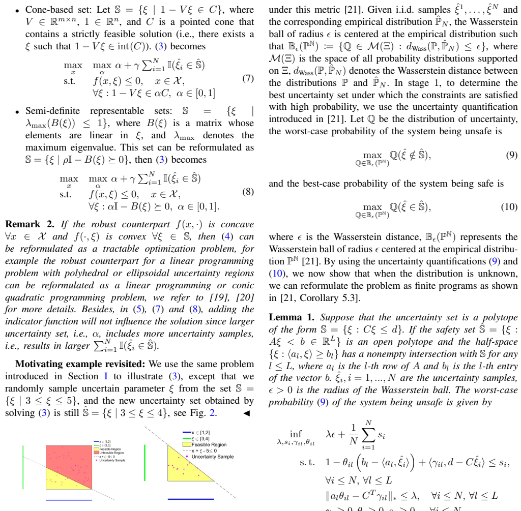
The central object is the scaled adjustable uncertainty set $\hat{S}(\alpha,v)=\{\xi: V\xi \le \alpha\mathbf{1}+(1-\alpha)Vv,\ Vv\le \mathbf{1},\ \alpha\in[0,1]\}$, where $\alpha$ shrinks the base polytope $\{V\xi\le\mathbf{1}\}$ toward a vertex $v$; the same parametric shrink is used for norm balls, cones, and semidefinite-representable sets. The second load-bearing mechanism is the Wasserstein ambiguity set $B_\epsilon(P_N)$, the ball of distributions within transportation distance $\epsilon$ of the empirical distribution of the samples. Lemma 1 uses the dual formulation of Wasserstein chance constraints to evaluate $\max_{Q\in B_\epsilon(P_N)}Q(\hat{\xi}\notin\hat{S})$ and $\max_{Q\in B_\epsilon(P_N)}Q(\hat{\xi}\in\hat{S})$ as finite optimizations, and Proposition 1 embeds those evaluations into the set-selection problem so that stage one is a finite program for polytopic uncertainty.
What would settle it
Re-run the numerical example of Section IV.A.2 and the power-flow study with the stage-one objective replaced by the worst-case unsafe probability $\min \sup_{Q\in B_\epsilon(P_N)}Q(\xi\notin\hat{S})$; if the chosen uncertainty sets are materially smaller or no feasible set exists for the same $N$ and $\epsilon$, the reported feasibility-preserving behavior depends on the optimistic objective and does not extend to a worst-case safety guarantee.
Extended reading notes
Core claim
The paper's claim is that feasibility should be treated as a design variable: when the original robust problem is infeasible under the full uncertainty set $S$, the decision-maker should choose the largest subset $\hat{S}\subseteq S$ for which a robustly feasible decision exists, using data to decide where to cut. The objective of this first stage is $\max_{x,\hat{S}}\mu(\hat{S})+\gamma\sum_{i=1}^{N}\mathbb{I}(\hat{\xi}_i\in\hat{S})$, where $\mu$ ranks sets and the penalty rewards covering the observed samples. In the stochastic case the same logic is applied with $\mu(\hat{S})$ replaced by an uncertainty-quantified probability over a Wasserstein ball; Lemma 1 converts the worst-case unsafe probability and the best-case safe probability into finite dual programs when $\hat{S}$ is a polytope, and Proposition 1 builds the stage-one reformulation for scaled polytopic sets. The paper asserts that this construction enlarges the feasible state set at the expense of a possible constraint violation, and reports concrete adjusted uncertainty sets and solutions for the power flow case.
Load-bearing premise
The stochastic stage chooses the uncertainty set by maximizing the best-case safe probability $\sup_{Q\in B_\epsilon(P_N)}Q(\xi\in\hat{S})$; because this is an optimistic upper bound, the claimed safety performance rests on using that particular objective rather than the worst-case probability of violation.
Editorial extensions
If this is right
- A robust problem that is infeasible under the original $S$ can still admit a decision once $\hat{S}$ is chosen as the largest feasible data-supported subset.
- The same scaling trick applies across the standard uncertainty-set families, so the method is not tied to a single geometry.
- For polytopic uncertainty and Wasserstein ambiguity, the first-stage set selection is a finite optimization problem rather than an infinite-dimensional one.
- In the optimal power flow case, the uncertainty in inertia can be narrowed to an interval that preserves the frequency constraints and yields a feasible dispatch.
Reading between the lines
- Beyond the paper: because the stochastic stage maximizes the best-case safe probability, the reported uncertainty sets are optimistic; replacing that objective with the worst-case unsafe probability would likely produce smaller sets for the same samples and radius.
- Beyond the paper: iterating the two stages, rather than stopping after one shrinkage, could converge to a minimal uncertainty set consistent with a required safety level; the paper does not analyze such a fixed point.
- Beyond the paper: a natural testable extension is to use the closed-polytope form of Lemma 1 to enforce a lower bound on the worst-case safe probability, turning the method into a calibrated chance-constrained design rather than an optimism-based one.
Editorial analysis
A structured set of objections, weighed in public.
Referee Report
Summary. The paper proposes a two-stage data-driven adjustable robust optimization method. In the first stage, the decision maker selects a subset of a nominal uncertainty set so that a robustly feasible decision exists while the subset is as large as possible and covers as many training samples as possible; in the second stage, the original objective is minimized over that selected subset. For non-stochastic uncertainty, the paper derives reformulations for norm-balls, ellipsoids, polyhedral sets, cone-based sets, and semi-definite representable sets. For stochastic uncertainty with unknown distribution, the paper uses a Wasserstein ambiguity set around the empirical distribution and invokes results from Mohajerin Esfahani and Kuhn to reformulate the stage-one problem, claiming a finite program for polytopic uncertainty sets. The proposed approach is illustrated on a simple numerical example and on an optimal power flow problem.
Significance. If the stochastic formulation were corrected, the paper would make a useful contribution: the non-stochastic part is a coherent and practically motivated way to trade off feasibility against sample coverage, and the power-system case study is a relevant application. The paper also draws a clear connection between adjustable robust optimization and data-driven set construction for several common uncertainty representations. However, the stochastic half currently uses an optimistic safety objective, and the finite-program reformulation contains inconsistencies, so the claimed distributionally robust guarantees are not established as written. These are correctable but load-bearing issues.
major comments (4)
- [§III, Eq. (13)-(15) and §IV.A.2, §IV.B.2] The stochastic stage uses the best-case safe probability max_{Q in B_epsilon(P_N)} Q(xi in S_hat) as the objective in the numerical experiments. This quantity is an optimistic upper bound: it can be large even if most distributions in the ambiguity ball make the selected set unsafe, and maximizing it does not control the violation probability under the true distribution or under an adversarial Q. The appropriate distributionally robust objective is to minimize the worst-case unsafe probability (9), whose finite reformulation is (14). As the experiments in Section IV.A.2 and IV.B.2 maximize the best-case branch, the reported uncertainty sets do not support the claimed performance guarantees for a robust scheme. The authors should rerun the stochastic experiments with the worst-case objective, or clearly reframe the contribution as a best-case analysis without DRO guarantees.
- [Proposition 1, Eq. (14)] The finite-program reformulation (14) is not well defined as written. The first constraint contains [1 + (1-alpha)V v]_l, but the proof in Eq. (16) and the substitution b = alpha 1 + (1-alpha)V v require [alpha 1 + (1-alpha)V v]_l. In addition, the dual-norm constraint uses a_l and C, which are not defined in the proposition; after substitution they should be V_l and V, respectively. The same applies to (15), where the matrix A in the dual-norm constraint is undefined. Until these substitutions are corrected, the proposition does not provide a valid finite reformulation.
- [Section III and Proposition 1, 'finite program' claim] The abstract and introduction state that for polytope uncertainty sets the problem can be reformulated as a finite program. However, the reformulations (14)-(15) only give a finite representation of the probability term; the constraint f(x, xi) <= 0 for all xi in S_hat remains a semi-infinite constraint. No general robust-counterpart reformulation for this constraint is provided in the proposition. To substantiate the finite-program claim, the authors need to impose and state additional structure on f (such as concavity in xi, as hinted in Remark 2) and give the corresponding tractable reformulation, or qualify the claim accordingly.
- [Lemma 1 and Proposition 1] The application of Lemma 1 to Proposition 1 is not consistent with the set assumptions. Lemma 1 states that formula (12) applies to a closed safety set S_hat = {xi : A xi <= b}, while Proposition 1 defines S_hat(alpha, v) = {xi : V xi < alpha 1 + (1-alpha)V v} with strict inequalities, i.e., an open set. The paper uses (12) in (15) for this open set without comment. The difference between open and closed polytopes matters for Wasserstein ambiguity set probabilities and for whether the reformulation is valid; the authors should either use the appropriate open-set formula or justify the substitution.
minor comments (6)
- [Eq. (8)] The text preceding (8) uses the symbol rho in the reformulation S = {xi : rho I - B(xi) >= 0}, but the constraint in (8) uses alpha I - B(xi) >= 0. Please unify the notation.
- [Eq. (6) and Prop. 1] The dimensions of V are inconsistent across the paper: in (6) V is described as an m by n matrix and 1 is an n-vector, while in Proposition 1 (14) the same V appears with inequalities V xi <= alpha 1 + (1-alpha)V v and V v <= 1, and the number of rows is later identified with L. Please align the notation and state the dimensions consistently.
- [Remark 2] The statement that adding the indicator function will not influence the solution under the assumption that a larger alpha gives a larger set is valid for the families (5), (7), and (8), but it is not generally true for the polyhedral family (6), where the set depends on both alpha and v and monotonicity in alpha is not guaranteed. Please qualify the remark.
- [Section IV.A.1] The solution is reported as v* = 10, but v is a vector in R^2 for the two-dimensional example. This appears to be a typo; please report the full vector.
- [Table I] The table reports 'new uncertainty set' intervals for different N and epsilon, but it does not state which stage-one objective (best-case or worst-case) was used. Since the text says the experiments use the best-case probability, this should be stated in the caption so the reader can interpret the numbers.
- [Section IV.B] The case study is described as a modified IEEE 5-bus system, but reference [23] points to a 14-bus test case archive. Please provide a specific citation for the 5-bus data or clarify the modification sources.
Circularity Check
No significant circularity: the two-stage programs are self-contained optimizations, and the Wasserstein duality is imported from an external theorem rather than from the paper's own assumptions.
full rationale
The derivation chain is self-contained and no load-bearing step reduces to its own inputs. The first-stage program (3) maximizes μ(Ŝ)+γΣ_i I(ξ̂_i∈Ŝ) subject to f(x,ξ)≤0 for all ξ∈Ŝ; this is a well-defined optimization over (x,Ŝ), and the second stage (4) solves a standard robust problem on the optimizer Ŝ. The non-stochastic specializations (5)-(8) are direct scalings of norm-ball, polyhedral, cone, and SDP-representable sets; the sample penalty is an extra term, not a hidden fit. The stochastic stage imports the Wasserstein duality formulas (11)-(12) from the external reference [21, Cor. 5.3] (Esfahani and Kuhn), and Proposition 1 substitutes the parametric polytope Ŝ(α,v) into those formulas. That substitution is derivativeness, not circularity: the reformulated finite program is obtained by epigraph manipulation of an external duality theorem, and the optimal α and v are the outcome of the program, not pre-imposed. The self-references [16]-[18] are related-work comparisons and are not used to justify the main result. Two non-circular technical concerns should be weighed separately: Eq. (14) appears to contain a typo, writing [1+(1−α)Vv]_l where Lemma 1 requires [α1+(1−α)Vv]_l, and A and C are not explicitly defined in Proposition 1; moreover, the stochastic experiments maximize the best-case safe probability sup_Q Q(ξ∈Ŝ) (Eqs. (21) and IV.B.2), which is an optimistic quantity and does not by itself certify a low worst-case violation probability. These are correctness or modeling risks, not circular reductions, so the circularity score is 0.
Assumptions & free parameters
free parameters (2)
- gamma (sample-coverage penalty weight) =
not reported
- Wasserstein radius epsilon =
0.05 and 0.1 in experiments
assumptions (3)
- domain assumption The uncertainty samples are i.i.d. from an unknown distribution P when the uncertainty is stochastic, and the empirical distribution with a Wasserstein ball is a valid model for P.
- domain assumption Lemma 1's conditions hold for the optimized sets: the open or closed polytope safety set has nonempty intersection with S, and each defining half-space has nonempty intersection with S.
- domain assumption The function f(x,.) is concave for each x and f(.,xi) is convex for each xi, so the robust counterpart can be reformulated tractably.
Cite this review
Pith. "Pith review of Data-Driven Adjustable Robust Optimization." pith.science (2026). https://pith.science/paper/HSMCGJF2
@misc{pith2026250522075,
  author       = {Pith},
  title        = {Pith review of: Data-Driven Adjustable Robust Optimization},
  year         = {2026},
  howpublished = {\url{https://pith.science/paper/HSMCGJF2}},
  note         = {Machine review of arXiv:2505.22075}
}
read the original abstract
In this paper, we develop a two-stage data-driven approach to address the adjustable robust optimization problem, where the uncertainty set is adjustable to manage infeasibility caused by significant or poorly quantified uncertainties. In the first stage, we synthesize an uncertainty set to ensure the feasibility of the problem as much as possible using the collected uncertainty samples. In the second stage, we find the optimal solution while ensuring that the constraints are satisfied under the new uncertainty set. This approach enlarges the feasible state set, at the expense of the risk of possible constraint violation. We analyze two scenarios: one where the uncertainty is non-stochastic, and another where the uncertainty is stochastic but with unknown probability distribution, leading to a distributionally robust optimization problem. In the first case, we scale the uncertainty set and find the best subset that fits the uncertainty samples. In the second case, we employ the Wasserstein metric to quantify uncertainty based on training data, and for polytope uncertainty sets, we further provide a finite program reformulation of the problem. The effectiveness of the proposed methods is demonstrated through an optimal power flow problem.
Figures


Reference graph
Works this paper leans on
-
[1]
Robust optimization–a comprehensive survey,
H.-G. Beyer and B. Sendhoff, “Robust optimization–a comprehensive survey,”Computer methods in applied mechanics and engineering, vol. 196, no. 33-34, pp. 3190–3218, 2007
work page 2007
-
[2]
Theory and applica- tions of robust optimization,
D. Bertsimas, D. B. Brown, and C. Caramanis, “Theory and applica- tions of robust optimization,”SIAM review, vol. 53, no. 3, pp. 464–501, 2011
work page 2011
-
[3]
M. B. Saltık, L. ¨Ozkan, J. H. Ludlage, S. Weiland, and P. M. Van den Hof, “An outlook on robust model predictive control algorithms: Reflections on performance and computational aspects,”Journal of Process Control, vol. 61, pp. 77–102, 2018
work page 2018
-
[4]
Robust optimization in power systems: a tutorial overview,
A. J. Conejo and X. Wu, “Robust optimization in power systems: a tutorial overview,”Optimization and Engineering, vol. 23, no. 4, pp. 2051–2073, 2022
work page 2022
-
[5]
C. Ning and F. You, “Optimization under uncertainty in the era of big data and deep learning: When machine learning meets mathemat- ical programming,”Computers & Chemical Engineering, vol. 125, pp. 434–448, 2019
work page 2019
-
[6]
From data to decisions: Distributionally robust optimization is optimal,
B. P. Van Parys, P. M. Esfahani, and D. Kuhn, “From data to decisions: Distributionally robust optimization is optimal,”Management Science, vol. 67, no. 6, pp. 3387–3402, 2021
work page 2021
-
[7]
N. Jiang and W. Xie, “Distributionally favorable optimization: A framework for data-driven decision-making with endogenous outliers,” SIAM Journal on Optimization, vol. 34, no. 1, pp. 419–458, 2024
work page 2024
-
[8]
Large-scale methods for distributionally robust optimization,
D. Levy, Y . Carmon, J. C. Duchi, and A. Sidford, “Large-scale methods for distributionally robust optimization,”Advances in Neural Information Processing Systems, vol. 33, pp. 8847–8860, 2020
work page 2020
Show all 24 references
-
[9]
Distributionally robust optimization: A review on theory and applications,
F. Lin, X. Fang, and Z. Gao, “Distributionally robust optimization: A review on theory and applications,”Numerical Algebra, Control and Optimization, vol. 12, no. 1, pp. 159–212, 2022
2022
-
[10]
On the road between robust optimization and the scenario approach for chance constrained optimization problems,
K. Margellos, P. Goulart, and J. Lygeros, “On the road between robust optimization and the scenario approach for chance constrained optimization problems,”IEEE Transactions on Automatic Control, vol. 59, no. 8, pp. 2258–2263, 2014
2014
-
[11]
Data-driven robust optimiza- tion,
D. Bertsimas, V . Gupta, and N. Kallus, “Data-driven robust optimiza- tion,”Mathematical Programming, vol. 167, pp. 235–292, 2018
2018
-
[12]
Wasserstein distributionally robust optimization: Theory and appli- cations in machine learning,
D. Kuhn, P. M. Esfahani, V . A. Nguyen, and S. Shafieezadeh-Abadeh, “Wasserstein distributionally robust optimization: Theory and appli- cations in machine learning,” inOperations research & management science in the age of analytics, pp. 130–166, 2019
2019
-
[13]
Nonparametric estimation of uncertainty sets for robust optimization,
P. Alexeenko and E. Bitar, “Nonparametric estimation of uncertainty sets for robust optimization,” in59th IEEE Conference on Decision and Control, pp. 1196–1203, 2020
2020
-
[14]
Satisficing models under uncertainty,
P. Jaillet, S. D. Jena, T. S. Ng, and M. Sim, “Satisficing models under uncertainty,”INFORMS Journal on Optimization, vol. 4, no. 4, pp. 347–372, 2022
2022
-
[15]
Robust optimal control with adjustable uncertainty sets,
X. Zhang, M. Kamgarpour, A. Georghiou, P. Goulart, and J. Lygeros, “Robust optimal control with adjustable uncertainty sets,”Automatica, vol. 75, pp. 249–259, 2017
2017
-
[16]
Robust risk-aware model predictive control of linear systems with bounded disturbances,
Y . Gao, C. Liu, and K. H. Johansson, “Robust risk-aware model predictive control of linear systems with bounded disturbances,” in IEEE 61st Conference on Decision and Control, pp. 1148–1155, 2022
2022
-
[17]
Opportunistic safety outside the maximal controlled invariant set,
Z. Liu, H. Chen, Y . Gao, and N. Ozay, “Opportunistic safety outside the maximal controlled invariant set,”IEEE Control Systems Letters, 2023
2023
-
[18]
Learning-based rigid tube model predictive control,
Y . Gao, S. Yan, J. Zhou, M. Cannon, A. Abate, and K. H. Johansson, “Learning-based rigid tube model predictive control,” in6th Annual Learning for Dynamics & Control Conference, pp. 492–503, 2024
2024
-
[19]
Robust optimization,
A. Ben-Tal, A. Nemirovski, and L. El Ghaoui, “Robust optimization,” 2009
2009
-
[20]
Deriving robust counter- parts of nonlinear uncertain inequalities,
A. Ben-Tal, D. Den Hertog, and J.-P. Vial, “Deriving robust counter- parts of nonlinear uncertain inequalities,”Mathematical programming, vol. 149, no. 1, pp. 265–299, 2015
2015
-
[21]
Data-driven distributionally robust optimization using the wasserstein metric: Performance guar- antees and tractable reformulations,
P. Mohajerin Esfahani and D. Kuhn, “Data-driven distributionally robust optimization using the wasserstein metric: Performance guar- antees and tractable reformulations,”Mathematical Programming, vol. 171, no. 1, pp. 115–166, 2018
2018
-
[22]
On the implementation of an interior- point filter line-search algorithm for large-scale nonlinear program- ming,
A. W ¨achter and L. T. Biegler, “On the implementation of an interior- point filter line-search algorithm for large-scale nonlinear program- ming,”Mathematical programming, vol. 106, pp. 25–57, 2006
2006
-
[23]
Power systems test case archive
“Power systems test case archive.”https://labs.ece.uw.edu/ pstca/pf14/pgn_tca14bus.htm, 1993. Accessed: Oct. 23, 2020
1993
-
[24]
Matpower 5.0 documentation
“Matpower 5.0 documentation.”https://matpower.org/ docs/ref/menu5.0.html. Accessed: Oct. 23, 2020
2020
Reviewed August 7, 2026 · model on record in the stance chip above.
Discussion (0). Sign in to comment.