REVIEW 3 major objections 4 minor 52 references
Hyperbolic polytrope
T0 review · 3 major / 4 minor · reviewed 2026-08-07 · deepseek-v4-flash
Pith's one-line read Polytropic fluids in hyperbolic symmetry are shown to yield bounded interior models that can source the vacuum inside a black-hole horizon.
desk verdict Solid first derivation of the hyperbolic Lane-Emden system, but the compactness upper bound is an artifact of the arbitrary inner boundary choice. read the letter →
The pith
A machine-rendered reading of the paper's core claim, the machinery that carries it, and where it could break.
The reading
What carries the argument
The central object is the Lane-Emden system for hyperbolically symmetric polytropes - Eqs. (43)-(44) for polytropic exponent $\gamma \neq 1$ and Eqs. (56)-(57) for $\gamma = 1$ - expressed in the dimensionless variables $\omega$, $\eta$, $x$ defined through Eqs. (38)-(42) and (54)-(55). The system is underdetermined until the anisotropy is specified; the paper closes it with the Cosenza-Herrera-Esculpi-Witten (CHEW) ansatz, Eq. (63), which expresses the anisotropy $\Pi = P_r - P_\perp$ in terms of $P_r - |\mu|$ and the metric function $\nu'$, controlled by a constant parameter $h$. This reduces the problem to a pair of first-order ODEs for $\omega$ and $\eta$, which are integrated numerically. The compactness $y = M/r_{\Sigma_e}$ then follows from the boundary value of $\eta$ through $y = q(n+1)\eta(x_{\Sigma_e})/x_{\Sigma_e}$.
What would settle it
A direct numerical check: for $h=0.9$, $q=0.1$, $n=20$ (beyond the plotted range), integrate Eqs. (64) and (44) from $x_{\Sigma_i}=0.1$ with the paper's boundary data and compute $y$ from Eq. (52); if $y$ continues to grow with $n$ rather than approaching $1/2$, or if $\omega$ fails to reach zero at the outer surface, the claimed upper bound and asymptotic behavior are wrong.
Extended reading notes
Core claim
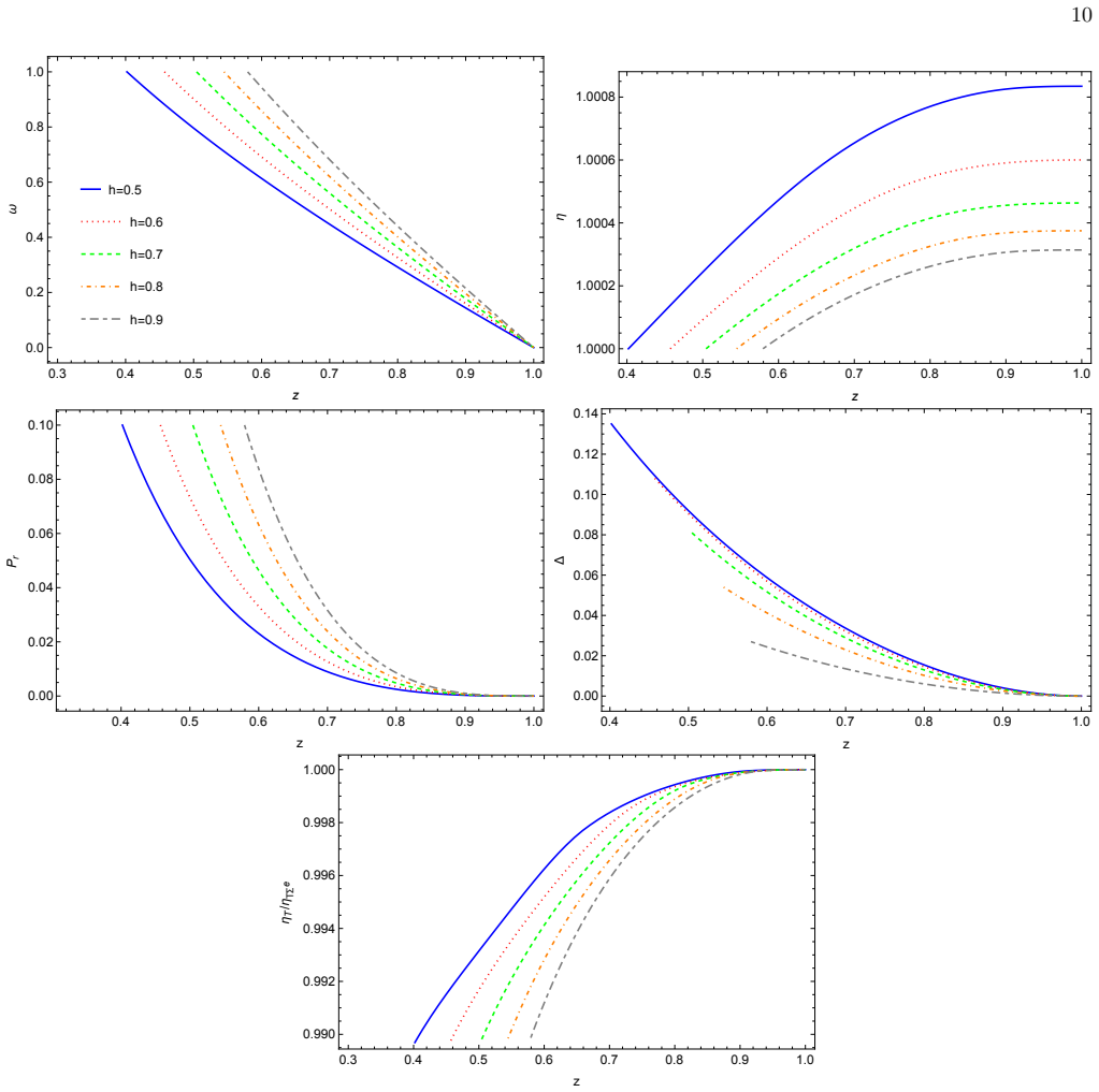
The paper claims that a static, locally anisotropic, polytropic fluid shell with hyperbolic symmetry can serve as the matter source of the interior hyperbolic vacuum. Working with the line element $ds^2 = e^{\nu}dt^2 - e^{\lambda}dr^2 - r^2(d\theta^2 + \sinh^2\theta\, d\phi^2)$, it reduces the structure equations to a Lane-Emden system, Eqs. (43)-(44) for $\gamma \neq 1$ and (56)-(57) for $\gamma = 1$, and closes the system with the Cosenza-Herrera-Esculpi-Witten (CHEW) anisotropy ansatz. The numerical models satisfy the expected monotonicity: $|\mu|$ and $P_r$ fall from the inner to the outer boundary, $P_r$ and the anisotropy $\Delta$ vanish at the surface, the mass function grows outward, and the anisotropy is positive and decreasing. Compactness $y = M/r_{\Sigma_e}$ is always above $1/2$, converges to $1/2$ as $n \to \infty$, and peaks at a finite maximum around $y \approx 2$ for the studied parameters, so the objects remain bounded and match the hyperbolic vacuum consistently.
Load-bearing premise
The construction rests on assuming the Cosenza-Herrera-Esculpi-Witten anisotropy closure, Eq. (63), together with the chosen inner boundary data, and the authors note that an alternative conformally flat closure gave unsatisfactory results; if that closure is wrong, the reported profiles and compactness bound do not follow.
Editorial extensions
If this is right
- The hyperbolic vacuum inside the horizon (line element (2)) can be matched to a polytropic anisotropic fluid shell, providing the first concrete matter source for that region in the static-interior picture.
- Because the energy density is negative throughout, the weak energy condition is violated, yet the matter variables retain the monotonic behavior expected for a bounded object, with radial pressure and anisotropy vanishing at the outer surface.
- Compactness is always greater than $1/2$ and bounded above, with a maximum near $y \approx 2$ for small $q$ and moderate $n$; as $n \to \infty$, $y \to 1/2$, so hyperbolic polytropes never become arbitrarily compact.
- The solution forms a layered, gravastar-like spacetime: a central constant-density spherical fluid, the hyperbolic polytrope shell, the hyperbolic vacuum, and the outer Schwarzschild vacuum, with the layers meeting only along the axis $\theta = 0$.
Reading between the lines
- The reported upper bound on compactness may be specific to the CHEW closure; re-solving the same Lane-Emden system with other closures (vanishing complexity, double polytrope) would show whether a maximum near $y \approx 2$ is generic to hyperbolic polytropes.
- A radial stability analysis is a natural next step: the paper establishes static equilibrium but says nothing about whether these shells are stable; if the repulsive interior gravity destabilizes the configurations, the physical relevance of the models would be limited.
- In the $\gamma = 1$ case the normalized Tolman mass has a local maximum near the surface, marking a region where the strong energy condition holds; this feature could serve as a distinguishing signature if such interior layers are ever probed observationally.
Editorial analysis
A structured set of objections, weighed in public.
Referee Report
Summary. The paper extends the relativistic polytrope formalism to static, hyperbolically symmetric spacetimes of the type proposed as a global extension inside the Schwarzschild horizon. After writing the Einstein equations for the metric (3) and the anisotropic fluid (5), the authors introduce a signed polytropic constant to handle the negative energy density, define dimensionless variables, and derive Lane-Emden systems for both γ≠1 (Eqs. (43)-(44)) and γ=1 (Eqs. (56)-(57)). The systems are closed with the Cosenza-Herrera-Esculpi-Witten anisotropy ansatz (61), integrated numerically from an inner boundary xΣi=0.1 with fixed initial data, and the resulting density, pressure, mass, Tolman mass, and anisotropy profiles are displayed. The paper also derives Tolman-mass expressions and discusses a layered cavity+polytrope+vacuum interpretation, and it reports that the compactness y=M/rΣe has an upper bound near y∼2 as a function of the polytropic index.
Significance. If the framework is correct, it provides explicit fluid models that could act as sources for the hyperbolic vacuum inside the horizon, a regime with very few concrete interior solutions. The algebraic reduction to Lane-Emden form and the Tolman-mass formulas are useful, self-contained generalizations of standard anisotropic polytrope methods, and the paper is transparent about the need for an extra closure condition. The main weakness is the numerical section: the central quantitative claim, the compactness upper bound, rests on a single arbitrarily chosen inner boundary radius and on initial data that are never connected to the advertised cavity matching. The qualitative 'expected behavior' of the matter profiles is also largely a consequence of the chosen boundary conditions and the CHEW ansatz, so it is not an independent validation. The framework is nevertheless a promising contribution, provided the claims are properly scoped.
major comments (3)
- [§V and Fig. 6; Eq. (52)] The headline claim that the compactness y is bounded above (y∼2) is not established by the numerical study. All integrations start from xΣi=0.1 with ω(xΣi)=1 and η(xΣi)=1, and the inner matching conditions (25)-(27) are never imposed, so xΣi is a free parameter. Since y=q(n+1)η(xΣe)/xΣe, the result depends directly on that arbitrary choice. Near xΣi, Eq. (64) gives dω/dx ≈ −h(1−q)/[2q(n+1)x], so the first zero of ω scales as xΣe ≈ xΣi exp[2q(n+1)/(h(1−q))], and therefore y ≈ q(n+1) exp[−2q(n+1)/(h(1−q))]/xΣi, which diverges as xΣi→0. The maximum near y∼2 in Fig. 6 is thus an artifact of fixing xΣi=0.1, not a robust property of hyperbolic polytropes. The abstract and Conclusions should either remove the claimed upper bound or restrict it explicitly to the explored boundary data and show how it depends on xΣi.
- [§III.A, Eq. (38) and Eqs. (43)-(44)] The definition of the dimensionless density variable is internally inconsistent. Eq. (38) defines ω_n = |μ|/|μ_f|, but Eq. (44) uses dη/dx = x^2ω^n and Eq. (43) contains ω^{n+1}. For the Lane-Emden reduction to be correct, the variable must satisfy ω^n = |μ|/|μ_f| (equivalently, ω = (|μ|/|μ_f|)^{1/n}). With the printed definition, Eq. (44) would give dη/dx = x^2(|μ|/|μ_f|)^n, which does not follow from m′=−4πr^2μ. The notation in Eq. (38) should be corrected and made consistent throughout Section III.A.
- [§II and §VI] The paper repeatedly describes a complete layered spacetime (spherically symmetric cavity plus hyperbolic polytrope plus hyperbolic vacuum plus Schwarzschild vacuum), but the inner matching is never actually performed. Eqs. (25)-(27) express the cavity constants in terms of m(Σi), ν′(Σi), and rΣi, yet no numerical solution is checked against these conditions, and the free data xΣi=0.1, ω(xΣi)=1, η(xΣi)=1 are not derived from any cavity model. As a result, the paper demonstrates solutions of the closed Lane-Emden system with arbitrary initial data, not the existence of a physically matched composite spacetime. The Conclusions should distinguish the general framework from the specific models integrated here.
minor comments (4)
- [§V] The numerical method is not described: no integrator, tolerance, or convergence tests are reported, and the figures have no error estimates. Please add these details or clearly state that the plots are illustrative.
- [§V and §VI] The qualitative agreement with the 'expected behavior' (decreasing |μ| and Pr, increasing η, positive Δ) is largely a consequence of the chosen boundary data and the CHEW ansatz with the sign conventions of Eq. (61). It should be presented as a property of the models explored, not as an independent physical validation of the framework.
- [§III.A, Eq. (41)] The parameter q is defined in Eq. (41) as P_f^r/|μ_f| at an unspecified reference point r_f, but the Discussion states that q is 'defined by the quotient of the respective thermodynamic quantities between the two boundary surfaces.' Please clarify whether r_f is the inner boundary, the outer boundary, or an arbitrary point in the fluid.
- [§VI] The conformally flat closure is mentioned only briefly as giving unsatisfactory results, with no details. Since this claim motivates the choice of CHEW anisotropy, a short description of the failure (or a reference to a forthcoming treatment) would help the reader judge the robustness of the results.
Circularity Check
No significant circularity: the Lane-Emden system is derived from the field equations and the polytropic EOS; the CHEW closure is an openly declared ansatz, and no fitted parameter is relabeled as a prediction.
full rationale
The core derivation is self-contained. The Lane-Emden systems (43)-(44) and (56)-(57) are obtained by substituting the polytropic EOS (37) and the dimensionless variables (38)-(42), (54)-(55) into the structure equations (14) and (17); the resulting equations are not assumed among the inputs, so no self-definitional reduction occurs. The CHEW closure (61) is introduced openly as an ansatz, and the paper states it is used "for convenience"; the positivity and decrease of the anisotropy are therefore recognized model outputs of an explicitly chosen closure, not independent predictions obtained from fitted parameters. No parameters are fitted to any data, so the fitted-input-called-prediction pattern does not apply. The prior-work citations that set the hyperbolic-vacuum scene ([1], [3], [4]) are by Herrera and collaborators, not by the present authors, and the present authors' own polytrope citations ([31], [35], [45], [47]) serve only as background or future-work pointers; none carries the load of the Lane-Emden derivation or of the compactness calculation. The compactness curve y(n) in Fig. 6 is a numerical consequence of integrating from a fixed inner point xSigma_i = 0.1 over q in [0.1, 0.3], h = 0.9, and n <= 20; its sensitivity to the chosen inner radius and to the closure is a robustness/generality concern, not a circular equivalence. The paper's own admission that the conformally flat closure gave "not entirely satisfactory" results is a limitation of the model scan, not a circular step. Overall, the derivation chain does not reduce to its own inputs by construction.
Assumptions & free parameters
free parameters (5)
- polytropic index n =
1-5 in plots for γ≠1; not applicable for γ=1
- q =
0.1, 0.15, 0.2, 0.25, 0.3
- h =
0.5-0.95 for γ≠1; 0.75-0.95 for γ=1
- boundary radius xΣi =
0.1
- initial ω and η at xΣi =
ω=1, η=1 for γ≠1; ω=0, η=0.6 for γ=1
assumptions (5)
- domain assumption Hyperbolic symmetric static metric (3) and global staticity inside the horizon
- domain assumption Energy density μ is negative, with mass function m defined by Eq. (13) and m'>0 requiring μ≤0
- ad hoc to paper Polytropic equation of state Pr=K|μ|^γ with adjusted constant to keep pressure real
- ad hoc to paper Cosenza-Herrera-Esculpi-Witten anisotropy ansatz (61): Π = C(Pr-|μ|)ν'r/2 with constant h=1-2C
- domain assumption Fluid is bounded by an inner cavity (filled with Schwarzschild interior solution) and an outer hyperbolic vacuum; matching conditions (20)-(22)
Cite this review
Pith. "Pith review of Hyperbolic polytrope." pith.science (2026). https://pith.science/paper/BAN42KN7
@misc{pith2026250522383,
  author       = {Pith},
  title        = {Pith review of: Hyperbolic polytrope},
  year         = {2026},
  howpublished = {\url{https://pith.science/paper/BAN42KN7}},
  note         = {Machine review of arXiv:2505.22383}
}
abstract
In this work, we study self-gravitating objects that obey a polytropic equation of state in hyperbolic symmetry. Specifically, we describe in detail the steps to derive the Lane-Emden equation from the structure equations of the system. To integrate the equations numerically, we propose the Cosenza-Herrera-Esculpi-Witten anisotropy and study the cases $\gamma \ne 1$ and $\gamma = 1$ in the parameter space of the models. We find that the matter sector exhibits the usual and expected behavior for certain values in this parameter space: energy density (in absolute value) and radial pressure are decreasing functions and vanish at the surface, while the mass function is increasing toward the surface. We find that the anisotropy of the system is positive and decreasing, consistent with the behavior of the radial pressure, which reaches a local minimum at the surface (i.e., the pressure gradient is zero at the surface). We also study the compactness of the dense objects as a function of the polytropic index and obtain that it has an upper bound given by the maximum value it reaches for a certain $n$. Some extensions of the work and future proposals are discussed.
Figures


Figures from the paper (3 more)


Reference graph
Works this paper leans on
-
[1]
(23) In addition, the condition m(rΣi ) = 0 must be satisfied
An empty flat cavity eνs = eλs = 1. (23) In addition, the condition m(rΣi ) = 0 must be satisfied. From (13), this condition implies that eλ = −1, which contradicts (23). Moreover, this will imply that the metric signature for the hyper- bolic fluid becomes (+ , +, −, −). For these reasons we rule out this case
-
[2]
An isotropic fluid with constant density eνs = ˜A − B r 1 − r2 C 2 !2 , e −λs = 1 − r2 C 2 , (24) where the matching conditions leads to | ˜A| = eν(Σi)/2 4 m(Σi)(4 − 2rΣi ν′(Σi)) + rΣi (rΣi ν′(Σi) − 4) rΣi − m(Σi) , (25) |B| = eν(Σi)/2r3/2 Σi p 2m(Σi) − rΣi |ν′(Σi)| 4|rΣi − m(Σi)| , (26) C 2 = r3 Σ 2(rΣi − m(Σi)) . (27) 5 The metric (24) corresponds to th...
-
[3]
Geodesics of the hyperbolically symmetric black hole
L. Herrera, A. Di Prisco, J. Ospino and L. Wit- ten, Phys. Rev. D 101 (2020) no.6, 064071 doi:10.1103/PhysRevD.101.064071 [arXiv:2002.07586 [gr-qc]]
work page Pith review arXiv 2020
- [4]
-
[5]
L. Herrera and L. Witten, Adv. High Energy Phys. 2018 (2018), 3839103 doi:10.1155/2018/3839103 [arXiv:1806.07143 [gr-qc]]
work page Pith review arXiv 2018
-
[6]
Rosen, doi:10.1007/978-1-4684-0721-1 13
N. Rosen, doi:10.1007/978-1-4684-0721-1 13
-
[7]
C. Hansen and S. Kawaler Stellar Interiors: Physical Principles, Structure and Evolution (Springer Verlag, Berlin, 1994)
work page 1994
- [8]
Show all 52 references
-
[9]
Chandrasekhar, An Introduction to the Study of Stellar Structure (University of Chicago, Chicago, 1939)
S. Chandrasekhar, An Introduction to the Study of Stellar Structure (University of Chicago, Chicago, 1939)
1939
-
[10]
Kippenhahn and A
R. Kippenhahn and A. Weigert, Stellar Structure and Evolution (Springer Verlag, Berlin, 1990)
1990
-
[11]
Abell´ an, P
G. Abell´ an, P. Bargue˜ no, E Contreras and E. Fuenmayor, Int. J. Mod. Phys. D 29 2050082 (2020)
2020
-
[12]
Herrera, Phys
L. Herrera, Phys. Rev. D 101, 104024 (2020)
2020
-
[13]
Herrera and W
L. Herrera and W. Barreto, Phys. Rev. D 87, 087303, (2013)
2013
-
[14]
Abell´ an, E
G. Abell´ an, E. Fuenmayor and L. Herrera, Phys. Dark Univ. 28, 100549 (2020)
2020
-
[15]
Tooper, Astrophys
R. Tooper, Astrophys. J. 143, 465 (1966)
1966
-
[16]
Bludman, Astrophys
S. Bludman, Astrophys. J. 183, 637 (1973)
1973
-
[17]
Tooper, Astrophys
R. Tooper, Astrophys. J. 140, 434 (1964)
1964
-
[18]
Tooper, Astrophys
R. Tooper, Astrophys. J. 142, 1541 (1965)
1965
-
[19]
Herrera and W
L. Herrera and W. Barreto, Gen. Relativ. Gravit. 36, 127 (2004)
2004
-
[20]
X. Y. Lai and R. X. Xu, Astropart. Phys. 31, 128 (2009)
2009
-
[21]
Nilsson and C
U. Nilsson and C. Uggla, Ann. Phys. 286, 292 (2000)
2000
-
[22]
force” and con- tains two different contributions. The first one is the “passive gravitational
provides a detailed and comprehensive study on gen- eral relativistic polytropes for anisotropic fluids. Also, a very complete analysis with varied applications has been published a few years ago ([31, 32]) which includes a gen- eralized equation that has been used for various...
-
[23]
Maeda, T
H. Maeda, T. Harada, H. Iguchi and N. Okuyama, Phys. Rev. D 66, 027501 (2002)
2002
-
[24]
Ngubelanga, S.D
S.A. Ngubelanga, S.D. Maharaj, Eur. Phys. J. Plus 130, 211 (2015)
2015
-
[25]
Thirukkanesh and F
S. Thirukkanesh and F. C. Ragel, Pramana J. Phys. 78, 687 (2012)
2012
-
[26]
Herrera and W
L. Herrera and W. Barreto, Phys. Rev. D 88, 084022, (2013)
2013
-
[27]
Herrera, A
L. Herrera, A. Di Prisco, W. Barreto and J. Ospino, Gen. Relativ. Gravit. 46, 1827 (2014)
2014
-
[28]
Mardan, A
S.A. Mardan, A. A. Siddiqui, I. Noureen and R.N. Jamil, Eur. Phys. J. Plus 135, 3 (2020)
2020
-
[29]
Harko, M.K
T. Harko, M.K. Mak, Astrophys. Space Sci. 361, 283 (2016)
2016
-
[30]
Abell´ an, E
G. Abell´ an, E. Contreras, E. Fuenmayor and L. Herrerra, Phys. Dark Univ. 30, 100632 (2020)
2020
-
[31]
Bhatti, Z
M.Z. Bhatti, Z. Tariq, Phys. Dark Univ. 28, 100482 (2020)
2020
-
[32]
Su´ arez–Urango, J
D. Su´ arez–Urango, J. Ospino, H. Hern´ andez and L. Nu˜ nez,Eur . Phys .J. C 802, 176 (2022)
2022
-
[33]
Ramos, C
A. Ramos, C. Arias, E. Fuenmayor and E. Contreras, Eur. Phys. J. C 81, 203 (2021)
2021
-
[34]
Hern´ andez, D
H. Hern´ andez, D. Su´ arez–Urango and L. Nu˜ nez,Eur. Phys. J. C 81, 241 (2021). 15
2021
-
[35]
Le´ on, E
P. Le´ on, E. Fuenmayor and E. Contreras Phys. Rev. D 104, 044053 (2021)
2021
-
[36]
Ovalle, Phys
J. Ovalle, Phys. Rev. D 95, 104019 (2017)
2017
-
[37]
Feroze and A
T. Feroze and A. A. Siddiqui, Gen. Relativ. Gravit. 43, 1035 (2011)
2011
-
[38]
Mardan, A
S. Mardan, A. Asif, and I. Noureen, Eur . Phys .J. C 134, 1 (2019)
2019
-
[39]
Santana, E
D. Santana, E. Fuenmayor and E. Contreras, Eur. Phys. J. C 82, 703 (2022)
2022
-
[40]
Herrera, J
L. Herrera, J. Ospino and A. Di Prisco, Phys. Rev. D 77, 027502 (2008)
2008
-
[41]
which allows one to find anisotropic matter solutions from any known isotropic one, in the spherically sym- metric case. The basic ansatz of the method is based on a specific form of the anisotropy, more specifically it is assumed that −Π = ∆ = P⊥ − Pr = C(Pr − |µ|) ν′ 2 r, (6...
2022
-
[42]
P. O. Mazur and E. Mottola, Universe 9 (2023) no.2, 88 doi:10.3390/universe9020088 [arXiv:gr-qc/0109035 [gr- qc]]
2023 arXiv
-
[43]
Tolman, Phys
R. Tolman, Phys. Rev. 35, 875 (1930)
1930
-
[44]
Herrera, A
L. Herrera, A. Di Prisco, J. Hern´ andez-Pastora, and N. O. Santos, Phys. Lett. A 237, 113 (1998)
1998
-
[45]
Cosenza, L
M. Cosenza, L. Herrera, M. Esculpi, L. Witten, J. Math. Phys. 22, 118 (1981)
1981
-
[46]
Herrera, A
L. Herrera, A. Di Prisco, J. Ospino, and E. Fuenmayor, J. Math. Phys. (N.Y.) 42, 2129 (2001)
2001
-
[47]
Herrera, Phys
L. Herrera, Phys. Rev. D 97, 044010 (2018)
2018
-
[48]
Bargue˜ no, E
P. Bargue˜ no, E. Fuenmayor and E. Contreras, Annals Phys. 443, 169012 (2022)
2022
-
[49]
Contreras, E
E. Contreras, E. Fuenmayor2 and G. Abell´ an2, Eur. Phys. J. C. 82, 187 (2022)
2022
-
[50]
Ya. B. Zeldovich, Zh. Eksp. Teor. Fiz. 41, 1609 (1969) [Sov. Phys. JETP 14, 1143 (1962)]
1969
-
[51]
Arias, E
C. Arias, E. Contreras, E. Fuenmayor and A. Ramos, Ann. Phys. 436, 168671 (2022)
2022
-
[52]
K. R. Karmarkar, Proc. Indian Acad. Sci. A 27, 56 (1948)
1948
Reviewed August 7, 2026 · model on record in the stance chip above.
Discussion (0). Sign in to comment.