REVIEW 2 major objections 6 minor 49 references
A Synthetic Business Cycle Approach to Counterfactual Analysis with Nonstationary Macroeconomic Data
T0 review · 2 major / 6 minor · reviewed 2026-08-07 · deepseek-v4-flash
Pith's one-line read This paper argues that conventional synthetic control on nonstationary macroeconomic outcomes can yield spurious counterfactuals, and proposes a trend-cycle decomposition estimator that is asymptotically unbiased.
desk verdict The SBC idea is solid and worth reviewing, but the main theorem's proof rests on a perfect-fit assumption that contradicts the paper's own Lemma A.1. read the letter →
The pith
A machine-rendered reading of the paper's core claim, the machinery that carries it, and where it could break.
The reading
What carries the argument
The load-bearing object is the Hamilton-filter trend-cycle decomposition used in a divide-and-conquer estimator. Hamilton's filter defines the trend $\tau_{i,t}$ as the linear projection of $Y_{i,t}(0)$ on its own values $h$ periods earlier (plus a constant), and the cycle $c_{i,t}$ as the resulting forecast error; because the forecast error is stationary for unit-root and trend-stationary processes, the synthetic control step is run on stationary inputs. The SBC estimator then combines the treated unit's own extrapolated trend with a synthetic cycle $\sum_{i=2}^{N+1}\hat{w}_i \hat{c}_{i,t}$, with weights fitted by matching pre-treatment cycles. The factor-structure assumption on cycles and the high-level consistency of the filter are what make the weighted cycle combination approximate the treated cycle, while the trend is kept separate precisely to avoid spurious regression.
What would settle it
Run a Monte Carlo design like Model 1 of the paper (independent random walks with drifts) with $T_0=200$, force the cycle-matching objective in equation (3) to a strictly positive minimum rather than zero, and record the bias of the SBC estimator at each post-treatment date. If the bias does not shrink as $T_0$ grows, the theorem's assumption of a perfect pre-treatment fit is doing the work and the asymptotic claim fails in that setting.
Extended reading notes
Core claim
The central claim is that the conventional synthetic control estimator can attribute common movement to treatment effects when outcomes contain unit-specific nonstationary trends, and that the correct division of labor is to trust the treated unit's own history for trend and the donor pool only for cycles. Formalized, the paper posits $Y_{i,t}(0)=\tau_{i,t}+c_{i,t}$ with stationary cycles $c_{i,t}=\lambda_i' f_t+\varepsilon_{i,t}$, and estimates the counterfactual as the treated unit's extrapolated trend plus a weighted average of donor cycles. Theorem 1 states that as the pre-treatment sample grows, the SBC estimator satisfies $\hat{Y}_{1,t}(0)-Y_{1,t}(0)=\sum_{i=2}^{N+1}\hat{w}_i(\varepsilon_{i,t}-\varepsilon_{1,t})+o_p(1)$, so the idiosyncratic part of the treated unit's cycle is the only asymptotic source of error and the estimator is asymptotically unbiased; without idiosyncratic shocks it is consistent. In the empirical illustrations, the SBC estimator produces counterfactuals that track placebo-period data while conventional synthetic control drifts, and the donor weights for trend and cycle select different countries.
Load-bearing premise
The proof of Theorem 1 assumes a perfect pre-treatment fit in the cycle-matching step: the treated unit's estimated cycle must be reproduced exactly by the donor cycle combination in every pre-treatment period, which is impossible when idiosyncratic shocks are present, and the asymptotic unbiasedness expansion depends on this cancellation.
Editorial extensions
If this is right
- A good pre-treatment fit by conventional synthetic control on nonstationary outcomes is not evidence that the counterfactual is valid; a placebo test with a shifted event date can expose the spurious drift.
- The SBC estimator is asymptotically unbiased for each post-treatment counterfactual period as the pre-treatment sample grows, regardless of whether the treated unit's trend is cointegrated with donor trends.
- When cycles follow an exact low-dimensional factor structure with no idiosyncratic shocks, the SBC estimator is consistent for the counterfactual outcome.
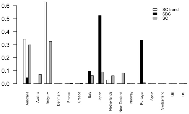
- In the paper's simulations, SBC cuts post-treatment mean-squared error relative to conventional synthetic control in spurious-trend designs, often by an order of magnitude under non-negative weights, and remains competitive when half the donors are cointegrated with the treated unit.
- In the German reunification and Hong Kong handover case studies, SBC assigns trend and cycle to different donor groups and yields a larger estimated treatment effect with placebo trajectories that stay close to actual data.
Reading between the lines
- An extension the authors leave implicit is inference: with multiple treated units or longer post-treatment windows, Theorem 1's characterization could be turned into confidence intervals for average treatment effects.
- The same trend-cycle split could be paired with other one-sided filters or model-based trend forecasts, which would make the approach robust to Hamilton filter misspecification.
- A testable prediction of the paper is that the gap between SBC and conventional synthetic control widens as the treated unit's nonstationary trend becomes more idiosyncratic relative to the donor pool.
- The placebo evidence suggests that outcome-only synthetic control applications on trending data should routinely report both trend and cycle weights, since the divergence itself diagnoses spurious matching.
Editorial analysis
A structured set of objections, weighed in public.
Referee Report
Summary. The paper proposes a synthetic control method for nonstationary panel outcomes, termed the synthetic business cycle (SBC) estimator. The procedure decomposes each unit's outcome into a trend and a cyclical component using the Hamilton filter, forecasts the treated unit's trend from its own history, and uses donor cycles to construct a synthetic cycle. The central theoretical claim (Theorem 1) is that the estimator is asymptotically unbiased for the counterfactual outcome under a factor structure for the cyclical components. The paper also provides Monte Carlo simulations and empirical applications to German reunification and the return of Hong Kong, where SBC is compared with a conventional synthetic control estimator.
Significance. The paper addresses a real and important gap: conventional synthetic control applied to nonstationary macroeconomic outcomes can produce spurious counterfactuals. The divide-and-conquer idea of separating trend and cycle is intuitive and economically motivated, and the simulation evidence is extensive and largely favorable to the proposed method. If the theoretical result were rigorously established, the paper would be a valuable contribution to the causal panel literature. The simulations and the two empirical illustrations are concrete strengths, as is the clear framing of the spurious synthetic control problem. However, the proof of the main theorem contains a substantial gap: it relies on an unstated perfect pre-treatment fit assumption that is not in the theorem's hypotheses and is inconsistent with a lemma proved in the same appendix. As a result, the central theoretical claim is not established in its current form.
major comments (2)
- [Appendix A, proof of Lemma A.1] The proof asserts 'we follow Abadie et al. (2010) in assuming a perfect pre-treatment fit, that is, the minimization problem in (3) attains zero.' This perfect-fit assumption is not part of Assumptions 1-2. With continuous idiosyncratic errors and T0 > N, exact equality of the estimated cycles is an event of probability zero. More importantly, Lemma A.1, proved in the same appendix, shows that the OLS weights converge to a limit that is generally not equal to the infeasible factor-matching weights w0. Consequently, the limiting weights do not satisfy Λ'_{-1}w∞ = λ1, and the factor mismatch term (λ1 - Σŵ_iλ_i)'f_t does not vanish in probability. The displayed substitution, which replaces F0λ1' - F0Σw_iλ_i' by idiosyncratic and estimation-error terms, is therefore invalid, and the asymptotic characterization Ŷ1,t(0)-Y1,t(0) = Σŵ_i(ε_i,t - ε_1,t) + op(1) does not follow. The theorem's claim of asymptotic unbiasedness may still be salvageable in a weaker, unconditional form when E[f_t]=0, but the proof as written does not establish the stated result under Assumptions 1-2.
- In deriving the probability limit of (1/˜T0)(Ĉ'_{-1})(ε_1 + û_1 - ε_{-1}w0 - û_{-1}w0), the term involving ε'_{-1}ε_{-1}w0 enters with a minus sign; the displayed expression in the manuscript retains a plus sign. Algebraically, ε'_{-1}(-ε_{-1}w0) = -ε'_{-1}ε_{-1}w0, so the limit is -Σε_{-1}w0, not +Σε_{-1}w0. This sign error affects the limiting weights derived in the lemma: the limit is shifted by a term involving Σε and is generally different from w0. The sign error reinforces the inconsistency with the perfect-fit substitution in Theorem 1 and means the lemma's statement, as written, is not correct.
minor comments (6)
- [Section 3.1, equation (2)] The coefficient αi2 should be αi,2, and the indexing of the lags is inconsistent: the regressors are Y_{t-h}, ..., Y_{t-h-p+1}, so the coefficient on the j-th lag should be αi,j.
- [Section 5.1] The conventional synthetic control comparison is based on a version without the covariates used by Abadie et al. (2015). The text acknowledges this, but the abstract and introduction may be read as directly challenging those estimates; please clarify the scope of the comparison.
- [Section 3.1] The method produces forecasts only for horizons up to h; the empirical figures should make clear that only these horizons are shown, or the paper should explain how longer-horizon forecasts would be obtained.
- [Section 3.3, Lemma 2] The statement of Lemma 2 is vague about the class of processes for which the projection coefficients are consistent; citing Hamilton (2018) without further justification may be insufficient for the nonstationary cases discussed.
- [Section 4, Table 1] The MSE ratios are reported without Monte Carlo standard errors, and some ratios are close to 1; reporting uncertainty in the simulation results would help assess whether small differences are meaningful.
- [Section 3.2, just before Theorem 1] The term 'unbiased' is used loosely: the estimator is defined for a fixed post-treatment t and unbiasedness is asymptotic; consider rephrasing to avoid confusion.
Circularity Check
No significant circularity: the synthetic business cycle counterfactual is an out-of-sample construction from the treated unit's own trend history and donor cycles, not a refit of the target outcome.
full rationale
The claimed derivation is not circular in the sense defined by the review protocol. The synthetic business cycle estimator separates the counterfactual into a trend component, obtained by extrapolating the treated unit's own pre-treatment history through the Hamilton filter (Eq. 2), and a cyclical component, imputed from donor cycles with weights fitted only to pre-treatment cyclical discrepancies (Eq. 3); the post-treatment object Yhat_1,t(0) = tauhat_1,t + chat_1,t is therefore an out-of-sample construction rather than a refit of the target. Theorem 1's asymptotic characterization is derived from explicit assumptions, namely the factor representation of cycles (Assumption 1), high-level filter-accuracy conditions (Assumption 2), and the standard perfect pre-treatment fit assumption attributed to Abadie et al. (2010); none of these inputs is the post-treatment outcome or an equivalent of it. The paper's self-citations (Phillips and Shi 2021; Mei, Phillips, and Shi 2024; Shi and Huang 2023; Hsiao, Shi, and Zhou 2022) are used as background or as discussion pointers, not as the load-bearing justification for the main identification. A technical concern exists in the proof: the perfect pre-treatment fit assumption appears inconsistent with the limiting-weight expression in Lemma A.1 when idiosyncratic errors are continuously distributed; however, that is a correctness and rigor issue, not a circular reduction of the prediction to its inputs. The empirical evaluations, with simulations based on known DGPs and placebo tests relative to external benchmarks, further indicate that the claimed advantages are not manufactured by the construction.
Assumptions & free parameters
free parameters (2)
- Hamilton filter horizon h =
2 in simulations; 4 in empirical applications
- Hamilton filter lag order p =
2 in all exercises
assumptions (3)
- domain assumption Cyclical components follow a common factor structure ci,t = lambda_i' ft + epsilon_i,t with bounded factors and positive definite factor second moments (Assumption 1).
- domain assumption Filter estimation error satisfies Assumption 2: pointwise op(1) and sum of squared errors op(T0).
- ad hoc to paper Perfect pre-treatment fit in the synthetic control minimization on cycles (Appendix A proof of Theorem 1).
Cite this review
Pith. "Pith review of A Synthetic Business Cycle Approach to Counterfactual Analysis with Nonstationary Macroeconomic Data." pith.science (2026). https://pith.science/paper/QPUDRPWV
@misc{pith2026250522388,
  author       = {Pith},
  title        = {Pith review of: A Synthetic Business Cycle Approach to Counterfactual Analysis with Nonstationary Macroeconomic Data},
  year         = {2026},
  howpublished = {\url{https://pith.science/paper/QPUDRPWV}},
  note         = {Machine review of arXiv:2505.22388}
}
read the original abstract
This paper investigates the use of synthetic control methods for causal inference in macroeconomic settings when dealing with possibly nonstationary data. While the synthetic control approach has gained popularity for estimating counterfactual outcomes, we caution researchers against assuming a common nonstationary trend factor across units for macroeconomic outcomes, as doing so may result in misleading causal estimation-a pitfall we refer to as the spurious synthetic control problem. To address this issue, we propose a synthetic business cycle framework that explicitly separates trend and cyclical components. By leveraging the treated unit's historical data to forecast its trend and using control units only for cyclical fluctuations, our divide-and-conquer strategy eliminates spurious correlations and improves the robustness of counterfactual prediction in macroeconomic applications. As empirical illustrations, we examine the cases of German reunification and the handover of Hong Kong, demonstrating the advantages of the proposed approach.
Figures


Figures from the paper (6 more)


Reference graph
Works this paper leans on
-
[1]
Abadie, A. (2021). Using synthetic controls: Feasibility, data requirements, and methodological aspects. Journal of Economic Literature\/ 59\/ (2), 391--425
work page 2021
-
[2]
Abadie, A., A. Diamond, and J. Hainmueller (2010). Synthetic control methods for comparative case studies: Estimating the effect of C alifornia’s tobacco control program. Journal of the American statistical Association\/ 105\/ (490), 493--505
work page 2010
-
[3]
Abadie, A., A. Diamond, and J. Hainmueller (2015). Comparative politics and the synthetic control method. American Journal of Political Science\/ 59\/ (2), 495--510
work page 2015
-
[4]
Abadie, A. and J. Gardeazabal (2003). The economic costs of conflict: A case study of the basque country. American Economic Review\/ 93\/ (1), 113--132
work page 2003
-
[5]
Acemoglu, D., S. Johnson, A. Kermani, J. Kwak, and T. Mitton (2016). The value of connections in turbulent times: Evidence from the united states. Journal of Financial Economics\/ 121\/ (2), 368--391
work page 2016
-
[6]
Andersson, J. J. (2019). Carbon taxes and CO _2 emissions: Sweden as a case study. American Economic Journal: Economic Policy\/ 11\/ (4), 1--30
work page 2019
- [7]
-
[8]
Asatryan, Z., C. Castell \'o n, and T. Stratmann (2018). Balanced budget rules and fiscal outcomes: Evidence from historical constitutions. Journal of Public Economics\/ 167 , 105--119
work page 2018
Show all 49 references
-
[9]
Bayati, N
Athey, S., M. Bayati, N. Doudchenko, G. Imbens, and K. Khosravi (2021). Matrix completion methods for causal panel data models. Journal of the American Statistical Association\/ 116\/ (536), 1716--1730
2021
-
[10]
Avila-Montealegre, O. and C. Mix (2024). Common trade exposure and business cycle comovement. Journal of International Economics\/ 152 , 103998
2024
-
[11]
Li, and M
Bai, C., Q. Li, and M. Ouyang (2014). Property taxes and home prices: A tale of two cities. Journal of Econometrics\/ 180\/ (1), 1--15
2014
-
[12]
Bai, J. (2009). Panel data models with interactive fixed effects. Econometrica\/ 77\/ (4), 1229--1279
2009
-
[13]
Bai, J. and S. Ng (2021). Matrix completion, counterfactuals, and factor analysis of missing data. Journal of the American Statistical Association\/ 116\/ (536), 1746--1763
2021
-
[14]
Pfeifer, and K
Becker, M., G. Pfeifer, and K. Schweikert (2021). Price effects of the austrian fuel price fixing act: a synthetic control study. Energy Economics\/ 97 , 105207
2021
-
[15]
Feller, and J
Ben-Michael, E., A. Feller, and J. Rothstein (2021). The augmented synthetic control method. Journal of the American Statistical Association\/ 116\/ (536), 1789--1803
2021
-
[16]
Beveridge, S. and C. R. Nelson (1981). A new approach to decomposition of economic time series into permanent and transitory components with particular attention to measurement of the ‘business cycle’. Journal of Monetary Economics\/ 7\/ (2), 151--174
1981
-
[17]
Billmeier, A. and T. Nannicini (2013). Assessing economic liberalization episodes: A synthetic control approach. Review of Economics and Statistics\/ 95\/ (3), 983--1001
2013
-
[18]
Botosaru, I. and B. Ferman (2019). On the role of covariates in the synthetic control method. The Econometrics Journal\/ 22\/ (2), 117--130
2019
-
[19]
Masini, and M
Carvalho, C., R. Masini, and M. C. Medeiros (2018). Ar C o: An artificial counterfactual approach for high-dimensional panel time-series data. Journal of Econometrics\/ 207\/ (2), 352--380
2018
-
[20]
Garcia, and L
Chamon, M., M. Garcia, and L. Souza (2017). FX interventions in B razil: A synthetic control approach. Journal of International Economics\/ 108 , 157--168
2017
-
[21]
Di Giovanni, J., A. A. Levchenko, and I. Mejean (2018). The micro origins of international business-cycle comovement. American Economic Review\/ 108\/ (1), 82--108
2018
-
[22]
Doudchenko, N. and G. W. Imbens (2016). Balancing, regression, difference-in-differences and synthetic control methods: A synthesis. Technical report, National Bureau of Economic Research
2016
-
[23]
crown jewel
Eliason, P. and B. Lutz (2018). Can fiscal rules constrain the size of government? A n analysis of the “crown jewel” of tax and expenditure limitations. Journal of Public Economics\/ 166 , 115--144
2018
-
[24]
Gobillon, L. and T. Magnac (2016). Regional policy evaluation: Interactive fixed effects and synthetic controls. Review of Economics and Statistics\/ 98\/ (3), 535--551
2016
-
[25]
Granger, C. W. and P. Newbold (1974). Spurious regressions in econometrics. Journal of Econometrics\/ 2\/ (2), 111--120
1974
-
[26]
Hamilton, J. D. (2018). Why you should never use the H odrick- P rescott filter. Review of Economics and Statistics\/ 100\/ (5), 831--843
2018
-
[27]
Hodrick, R. J. and E. C. Prescott (1997). Postwar us business cycles: an empirical investigation. Journal of Money, Credit, and Banking\/ 29\/ (1), 1--16
1997
-
[28]
Hou, L., K. Li, Q. Li, and M. Ouyang (2021). Revisiting the location of fdi in china: A panel data approach with heterogeneous shocks. Journal of Econometrics\/ 221\/ (2), 483--509
2021
-
[29]
Hsiao, C., S. H. Ching, and S. K. Wan (2012). A panel data approach for program evaluation: Measuring the benefits of political and economic integration of H ong K ong with mainland C hina. Journal of Applied Econometrics\/ 27\/ (5), 705--740
2012
-
[30]
Shi, and Q
Hsiao, C., Z. Shi, and Q. Zhou (2022). Transformed estimation for panel interactive effects models. Journal of Business & Economic Statistics\/ 40\/ (4), 1831--1848
2022
-
[31]
Ibragimov, R. and S. Sharakhmetov (2002). The exact constant in the rosenthal inequality for random variables with mean zero. Theory of Probability & Its Applications\/ 46\/ (1), 127--132
2002
-
[32]
Shen, and Q
Li, X., Y. Shen, and Q. Zhou (2024). Confidence intervals of treatment effects in panel data models with interactive fixed effects. Journal of Econometrics\/ 240\/ (1), 105684
2024
-
[33]
Masini, R. and M. C. Medeiros (2021). Counterfactual analysis with artificial controls: Inference, high dimensions, and nonstationarity. Journal of the American Statistical Association\/ 116\/ (536), 1773--1788
2021
-
[34]
Masini, R. and M. C. Medeiros (2022). Counterfactual analysis and inference with nonstationary data. Journal of Business & Economic Statistics\/ 40\/ (1), 227--239
2022
-
[35]
Mayoral, L. (2013). Heterogeneous dynamics, aggregation, and the persistence of economic shocks. International Economic Review\/ 54\/ (4), 1295--1307
2013
-
[36]
McCracken, M. W. and S. Ng (2016). FRED-MD : A monthly database for macroeconomic research. Journal of Business & Economic Statistics\/ 34\/ (4), 574--589
2016
-
[37]
Mei, Z., P. C. Phillips, and Z. Shi (2024). The boosted H odrick- P rescott filter is more general than you might think. Journal of Applied Econometrics\/ 39\/ (7), 1260--1281
2024
-
[38]
Seidel, F
Meinhardt, V., B. Seidel, F. Stille, and D. Teichmann (1995). Transferleistungen in die neuen bundesländer und deren wirtschaftliche konsequenzen. Sonderheft 154, Deutsches Institut für Wirtschaftsforschung (DIW Berlin), Berlin
1995
-
[39]
Miao, K., P. C. Phillips, and L. Su (2023). High-dimensional vars with common factors. Journal of Econometrics\/ 233\/ (1), 155--183
2023
-
[40]
Moon, H. R. and M. Weidner (2017). Dynamic linear panel regression models with interactive fixed effects. Econometric Theory\/ 33\/ (1), 158--195
2017
-
[41]
Onatski, A. and C. Wang (2021). Spurious factor analysis. Econometrica\/ 89\/ (2), 591--614
2021
-
[42]
Peri, G. and V. Yasenov (2019). The labor market effects of a refugee wave: Synthetic control method meets the mariel boatlift. Journal of Human Resources\/ 54\/ (2), 267--309
2019
-
[43]
Phillips, P. C. (1986). Understanding spurious regressions in econometrics. Journal of Econometrics\/ 33\/ (3), 311--340
1986
-
[44]
Phillips, P. C. and Z. Shi (2021). Boosting: W hy you can use the HP filter. International Economic Review\/ 62\/ (2), 521--570
2021
-
[45]
Shen, D., P. Ding, J. Sekhon, and B. Yu (2023). Same root different leaves: Time series and cross-sectional methods in panel data. Econometrica\/ 91\/ (6), 2125--2154
2023
-
[46]
Shi, Z. and J. Huang (2023). Forward-selected panel data approach for program evaluation. Journal of Econometrics\/ 234\/ (2), 512--535
2023
-
[47]
Stock, J. H. and M. W. Watson (1988). Variable trends in economic time series. Journal of Economic Perspectives\/ 2\/ (3), 147--174
1988
-
[48]
Stock, J. H. and M. W. Watson (1999). Business cycle fluctuations in US macroeconomic time series. Handbook of Macroeconomics\/ 1 , 3--64
1999
-
[49]
Xiong, R. and M. Pelger (2023). Large dimensional latent factor modeling with missing observations and applications to causal inference. Journal of Econometrics\/ 233\/ (1), 271--301
2023
Reviewed August 7, 2026 · model on record in the stance chip above.
Discussion (0). Sign in to comment.