REVIEW 3 major objections 5 minor 45 references
Kernel-Smoothed Scores for Denoising Diffusion: A Bias-Variance Study
T0 review · 3 major / 5 minor · reviewed 2026-08-07 · deepseek-v4-flash
Pith's one-line read A kernel-smoothed score provably reduces the dataset size at which a diffusion model switches from memorizing to generalizing, by convolving the empirical score with a Gaussian of bandwidth $h_N = t_N^\beta$.
desk verdict Solid CLT and bias-variance core, but the headline memorization-transition claim rests on an unproved uniformity in t that the authors themselves flag. read the letter →
The pith
A machine-rendered reading of the paper's core claim, the machinery that carries it, and where it could break.
The reading
What carries the argument
The central object is the mollified empirical score $\tilde s_t^N = G_h \star s_t^N$, the convolution of the empirical score with a Gaussian kernel of bandwidth $h$; because the Gaussian kernel is centered, this is also the score of the LED-KDE density $(G_h, G_t)\star p_0^N$. The argument runs on three pieces: a central limit theorem for the empirical score whose noise covariance is a re-weighted data PCA aligned with the tangent space; a bias-variance decomposition of the mollified score, with the variance term controlled by a Gaussian-process computation using Laplace's method and the bias controlled by the smoothing lengthscale; and a KL-divergence bound that converts score estimation error into distribution error. The bandwidth does the work: it suppresses the high-frequency components of the score without adding bias, effectively replacing a dataset of size $N$ by one of effective size $N_{\mathrm{eff}}\approx N(h/t)^{k/2}$.
What would settle it
Fix a known $k$-dimensional linear manifold with density $p_*$, draw $N$ samples, and measure the KL divergence between $G_{t_N} \star p_*$ and the law generated by the mollified reverse SDE for $t_N \to 0$ with $h_N = t_N^\beta$, $\beta \in (1/2,1)$. Theorem 4 predicts the divergence scales as $h_N^2/t_N + \log(1/t_N)/(N h_N^{k/2})$; if the data-dependent term instead scales like the unsmoothed bound $1/(N t_N^{k/2})$, or if the crossover sample size does not drop from $N_c = t_N^{-k/2}$ to about $N_c^\beta$, the central claim fails. A cheaper check: compare the empirical covariance of $\sqrt{N}(m_t^N(x)-m_t(x))$ to the predicted $t^{-k/2}P_{TM(x)}/p_*(\pi(x))$ at small times.
Extended reading notes
Core claim
Under the assumption that data lies on a smooth $k$-dimensional manifold (linear for the main theorems), the empirical score seen through its Gaussian approximation has covariance $\Sigma_{(t,x),(t,x)} \sim t^{-k/2} p_*(\pi(x))^{-1} P_{TM(x)}$, so the sampling noise lives in tangent directions and diverges at small times. Convolving with a Gaussian kernel of bandwidth $h_N$ turns the score into the score of the Log-Exponential Double-Kernel Density Estimator (LED-KDE), $(G_h, G_t) \star p_0^N$. The bias-variance decomposition gives variance of order $t_N/(N h_N^{k/2})$ and bias of order $h_N^2$, and the KL bound $\mathbb{E}_D D_{KL}(p_{t_N}\|\tilde q^N_{t_N}) = O(h_N^2/t_N + \log(1/t_N)/(N h_N^{k/2})) + D_{KL}(p_T\|N(0,T I_d))$ follows. With $h_N = t_N^\beta$, $\beta \in (1/2,1)$, the critical dataset size for the memorization-to-generalization transition drops from $N_c = t_N^{-k/2}$ to $\tilde N_c = N_c^\beta$. The paper also gives a spectral heuristic suggesting this bound can be improved with an adaptive lengthscale, and interprets the mollified reverse diffusion as a Wasserstein gradient flow attracted to a smoothed (LED-KDE) measure.
Load-bearing premise
The whole analysis relies on the sampling noise in the score being Gaussian even at the tiny times where memorization happens, but the paper only proves that Gaussian behavior for fixed positive times.
Editorial extensions
If this is right
- Convolving the score with a Gaussian kernel of appropriate bandwidth reduces the critical dataset size for the memorization-to-generalization transition from $N_c = t_N^{-k/2}$ to roughly $N_c^\beta$, so the same model generalizes from far fewer samples.
- Because smoothing suppresses the small-time divergence of the score noise, the reverse process can start from a smaller time $t_N$, limiting the initial Gaussian leakage of mass away from the data manifold.
- The paper's bounds suggest an effective dataset size $N_{\mathrm{eff}} \approx N(h/t)^{k/2}$, giving a quantitative target: at very small times, a regularized score built from $N$ points behaves like an unregularized score from a much larger sample.
- The mollified reverse SDE is the Wasserstein gradient flow of the KL divergence toward a smoothed (LED-KDE) measure, so even a fixed smoothing, with no learned model, acts as a generalization mechanism.
- The paper's spectral heuristic indicates that frequency truncation by the kernel could improve the KL bound to $O(t_N/(N h_N^{1+d/2}))$, suggesting that adaptive, time-dependent bandwidths can outperform the isotropic kernel analyzed in the theorems.
Reading between the lines
- Editorial inference: the same smoothing argument should transfer to pretrained score networks, not just the empirical score: convolving a network's output with a Gaussian kernel at generation time is a cheap post-hoc memorization mitigation, which the paper sketches but does not test.
- Editorial inference: the appendix's observation that mollification approximates evaluating the score at a larger time suggests that common sampling heuristics such as early stopping or coarser time steps already realize part of the smoothing benefit; a direct comparison between explicit kernel smoothing and time-step coarsening would test this.
- Editorial inference: because the score-noise covariance aligns with the data tangent space, an anisotropic or manifold-adapted kernel should control variance better than the isotropic Gaussian used in the theorems; a natural experiment is to replace $G_h$ by a kernel whose covariance follows the local empirical PCA and compare realized KL divergences.
- Editorial inference: the LED-KDE factorization implies the regularization effectively smooths along the intrinsic manifold, so the memorization threshold should depend on intrinsic dimension $k$ rather than ambient dimension $d$; this can be checked by embedding the same low-dimensional data in higher ambient spaces.
Editorial analysis
A structured set of objections, weighed in public.
Referee Report
Summary. The paper studies denoising diffusion models driven by the empirical score built from a finite dataset, and proposes a kernel-smoothed (mollified) empirical score as an analytically tractable proxy for the regularization induced by parametric score networks. The main theoretical results are: (i) a central limit theorem for the empirical conditional expectation m_t^N, with covariance asymptotics showing a small-time blow-up and decorrelation along a k-dimensional data manifold (Theorem 2); (ii) a bias-variance decomposition for the mollified score (Theorem 3); and (iii) upper bounds on the KL divergence between the true noised distribution p_{t_N} and the generated distributions for the empirical and mollified scores (Theorem 4), from which the authors conclude that smoothing changes the memorization-to-generalization transition from N_c = t_N^{-k/2} to roughly N_c^β. The paper also introduces the LED-KDE interpretation of the mollified score as a two-stage smoothing procedure and presents numerical experiments on Swiss-roll, MNIST, and synthetic manifolds.
Significance. If the bounds in Theorem 4 were fully rigorous, the paper would provide one of the few analytic handles on the memorization-generalization trade-off in diffusion models, with the striking and falsifiable prediction that explicit score smoothing behaves like an enlarged training set. The derivation of the covariance structure as a re-weighted local PCA, the LED-KDE reformulation, and the spectral heuristic are all interesting and potentially useful starting points for future work. The paper is also commendably transparent about its own limitations, and the appendices contain substantial derivations with standard tools (CLT, delta method, Laplace's method). The central caveat is that the headline phase-transition claim rests on a small-time uniformity that is neither stated nor proved; until that gap is addressed, the results should be viewed as conditional.
major comments (3)
- [§5.3, Theorem 4 and Appendix A.7] The bound (13) is obtained by integrating the small-time variance asymptotic over [t_N, T], but the underlying CLT (Theorem 2) is stated for fixed t > 0 and the Laplace expansions are not accompanied by a uniformity statement in t. As t -> 0, the denominator φ^(0)(t,x) is of order (2π t)^{k/2} p_*(π(x)), so after division by t^2 the omitted o(N^{-1/2}) terms have coefficients that diverge like t^{-(k/2+1)}. The transition scale N_c = t_N^{-k/2} is exactly the regime where N φ^(0) is O(1), where the CLT has no valid asymptotic margin. The authors acknowledge this in the Limitations section, but the acknowledgment does not remove the need for either a uniform CLT or a non-asymptotic bound in the relevant regime. As stated, (12)-(13) are conditional on an unproved uniformity assumption, and the headline transition claim rests on that assumption.
- [§5.3, Theorem 4 (12)-(13)] The 'transition' from memorization to generalization is inferred from where the right-hand sides of the upper bounds blow up, not from matching lower bounds. Even if the CLT uniformity issue were fixed, an upper bound alone does not establish that a sharp transition occurs at N_c or at N_c^β; it only shows that the bound is vacuous in the claimed regime. The text should either prove a lower bound (or a two-sided bound) or be reworded so that the phase-transition language is explicitly heuristic.
- [§5.2, Eq. (9) and Appendix A.4] The proof of Theorem 4 uses E[||m_t^N - m_t||^2] ≈ (1/N) tr Σ_{(t,x),(t,x)}. Theorem 2 establishes convergence in finite-dimensional distribution, not convergence of second moments; the latter requires uniform integrability, which is not shown and is plausible to fail at small t where the variance diverges. This is another load-bearing gap in the derivation of (12)-(13) that should be addressed or explicitly assumed.
minor comments (5)
- [§6, Discussion] The text refers to 'Theorem 14' when discussing the covariance matrix; this should be 'Theorem 2'.
- [§5.3, after Eq. (13)] The notation N_c^β ≪ N_c is used without defining the exponent domain in the main text; it is clear from context that β ∈ (1/2,1), but this should be restated at the point of use.
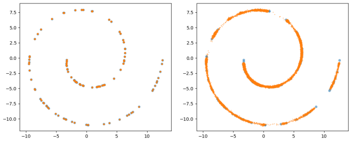
- [Figure 4 and Figure 10] The y-axis label 'Dataset ratio' is used in both figures; the text and captions define it as N_eff/N only in the body, but the figures themselves would benefit from the explicit definition in the axis label or caption.
- [Appendix A.7, proof of Theorem 4] The sentence 'which proves the claim, up to a non-important log 1/t_N factor' is inconsistent with the statement of Theorem 4, which includes the logarithmic factor; either the theorem or the proof annotation should be aligned.
- [Appendix A.10, spectral viewpoint] The notation f_k(x) := cos(π kx) is introduced for k ∈ N but then used as a multi-index k ∈ N^d; please clarify the multi-index convention at first use.
Circularity Check
No circularity: the KL bounds are derived from stated assumptions and standard probabilistic tools; the acknowledged CLT small-time limitation is a technical gap, not a circular step.
full rationale
The paper's derivation chain is self-contained and does not reduce its conclusions to its inputs. Theorem 2 derives a CLT for the empirical score from the classical CLT, Skorokhod representation, and a delta-method Taylor expansion. Theorem 3 computes the variance and bias of the mollified score from Theorem 2's covariance asymptotics and Laplace's method. Theorem 4 then combines the bias-variance decomposition with the standard KL bound of Song et al. (11). Each step uses stated assumptions, and no fitted parameter is renamed as a prediction. The replacement of the empirical score by its Gaussian approximation in (9) is explicitly flagged: 'we stress that the results below are valid up to the validity of the CLT.' The Limitations section repeats this condition: 'our analysis relies on the Gaussian approximation of m^N by the CLT of Theorem 2, which for a fixed N requires the time to not be too small.' The lack of a uniform CLT remainder as t goes to 0 is a genuine technical-rigor concern about the small-time regime, but it is an acknowledged assumption in the derivation, not a circular equivalence between the conclusion and the premise. The "transition scale" N_c is presented as a suggestion from where the upper bound blows up ('Inequality (12) suggests...', 'this indicates...'), not as a fitted claim. The effective dataset size N_eff is defined through the paper's own upper bounds and is described as a suggestion ('The upperbounds of the previous theorem suggest that N_eff ≈ N(h/t)^{k/2}'), and its numerical estimates are experiments, not inputs to the theorems. The spectral viewpoint is explicitly marked as heuristic: 'We stress that the approach below is heuristic while the other results of this work are rigorously established.' The only self-citation is [20] (Jacot, Gabriel, Hongler), used as heuristic motivation that wide NTK networks learn a kernel projection of the empirical score; this is not load-bearing for the paper's theoretical claims. Overall, no step of the derivation is equivalent to its inputs by construction.
Assumptions & free parameters
free parameters (2)
- kernel bandwidth h =
h = 0.75, 0.3, 0.2 and similar values in experiments; asymptotic form h = t^beta
- exponent beta =
beta in (1/2, 1)
assumptions (6)
- domain assumption The data distribution p* is supported on a smooth k-dimensional manifold with smooth density, uniformly bounded second derivatives, and p* > 0.
- domain assumption Assumption 1: the manifold M supporting p* is a k-dimensional linear subspace of R^d.
- domain assumption The empirical score is replaced by the Gaussian approximation m^N_t = m_t + G/sqrt(N).
- domain assumption Brownian noising with sigma = 1 is used; Ornstein-Uhlenbeck processes are excluded.
- domain assumption The KL divergence bound of Song et al. applies to the reverse SDE with estimated score.
- standard math Classical CLT, delta method, Fubini, and Laplace's method are valid for the quantities being expanded.
invented entities (1)
-
LED-KDE (Log-Exp Double-Kernel Density Estimator)
Cite this review
Pith. "Pith review of Kernel-Smoothed Scores for Denoising Diffusion: A Bias-Variance Study." pith.science (2026). https://pith.science/paper/7MHJFZN2
@misc{pith2026250522841,
  author       = {Pith},
  title        = {Pith review of: Kernel-Smoothed Scores for Denoising Diffusion: A Bias-Variance Study},
  year         = {2026},
  howpublished = {\url{https://pith.science/paper/7MHJFZN2}},
  note         = {Machine review of arXiv:2505.22841}
}
read the original abstract
Diffusion models now set the benchmark in high-fidelity generative sampling, yet they can, in principle, be prone to memorization. In this case, their learned score overfits the finite dataset so that the reverse-time SDE samples are mostly training points. In this paper, we interpret the empirical score as a noisy version of the true score and show that its covariance matrix is asymptotically a re-weighted data PCA. In large dimension, the small time limit makes the noise variance blow up while simultaneously reducing spatial correlation. To reduce this variance, we introduce a kernel-smoothed empirical score and analyze its bias-variance trade-off. We derive asymptotic bounds on the Kullback-Leibler divergence between the true distribution and the one generated by the modified reverse SDE. Regularization on the score has the same effect as increasing the size of the training dataset, and thus helps prevent memorization. A spectral decomposition of the forward diffusion suggests better variance control under some regularity conditions of the true data distribution. Reverse diffusion with kernel-smoothed empirical score can be reformulated as a gradient descent drifted toward a Log-Exponential Double-Kernel Density Estimator (LED-KDE). This perspective highlights two regularization mechanisms taking place in denoising diffusions: an initial Gaussian kernel first diffuses mass isotropically in the ambient space, while a second kernel applied in score space concentrates and spreads that mass along the data manifold. Hence, even a straightforward regularization-without any learning-already mitigates memorization and enhances generalization. Numerically, we illustrate our results with several experiments on synthetic and MNIST datasets.
Figures


Figures from the paper (11 more)




Reference graph
Works this paper leans on
-
[1]
Karim M Abadir and Jan R Magnus. Matrix algebra, volume 1. Cambridge University Press, 2005
work page 2005
-
[2]
Losing dimensions: Geometric memorization in generative diffusion, 2024
Beatrice Achilli, Enrico Ventura, Gianluigi Silvestri, Bao Pham, Gabriel Raya, Dmitry Krotov, Carlo Lucibello, and Luca Ambrogioni. Losing dimensions: Geometric memorization in generative diffusion, 2024
work page 2024
- [3]
-
[4]
Kovachki, Assad Oberai, and Andrew M
Ricardo Baptista, Agnimitra Dasgupta, Nikola B. Kovachki, Assad Oberai, and Andrew M. Stuart. Memorization and regularization in generative diffusion models, 2025
work page 2025
-
[5]
Carl M Bender and Steven A Orszag. Advanced mathematical methods for scientists and engineers I: Asymptotic methods and perturbation theory. Springer Science & Business Media, 2013
work page 2013
-
[6]
Dynamical regimes of diffusion models
Giulio Biroli, Tony Bonnaire, Valentin de Bortoli, and Marc Mézard. Dynamical regimes of diffusion models. Nature Communications, 15(1):9957, Nov 2024
work page 2024
-
[7]
Shallow diffusion networks provably learn hidden low-dimensional structure
Nicholas Matthew Boffi, Arthur Jacot, Stephen Tu, and Ingvar Ziemann. Shallow diffusion networks provably learn hidden low-dimensional structure. In The Thirteenth International Conference on Learning Representations, 2025
work page 2025
-
[8]
Swarm gradient dynamics for global optimization: the mean-field limit case
Jérôme Bolte, Laurent Miclo, and Stéphane Villeneuve. Swarm gradient dynamics for global optimization: the mean-field limit case. Mathematical Programming, 205(1):661–701, May 2024
work page 2024
Show all 45 references
-
[9]
Extracting training data from diffusion models
Nicholas Carlini, Jamie Hayes, Milad Nasr, Matthew Jagielski, Vikash Sehwag, Florian Tramèr, Borja Balle, Daphne Ippolito, and Eric Wallace. Extracting training data from diffusion models. In Proceedings of the 32nd USENIX Conference on Security Symposium, SEC ’23, USA, 2023. ...
2023
-
[10]
Towards memorization-free diffusion models, 2024
Chen Chen, Daochang Liu, and Chang Xu. Towards memorization-free diffusion models, 2024
2024
-
[11]
Improved analysis of score-based generative modeling: user-friendly bounds under minimal smoothness assumptions
Hongrui Chen, Holden Lee, and Jianfeng Lu. Improved analysis of score-based generative modeling: user-friendly bounds under minimal smoothness assumptions. In Proceedings of the 40th International Conference on Machine Learning, ICML’23. JMLR.org, 2023
2023
-
[12]
Score approximation, estimation and distribution recovery of diffusion models on low-dimensional data
Minshuo Chen, Kaixuan Huang, Tuo Zhao, and Mengdi Wang. Score approximation, estimation and distribution recovery of diffusion models on low-dimensional data. In Proceedings of the 40th International Conference on Machine Learning, ICML’23. JMLR.org, 2023
2023
-
[13]
On the interpolation effect of score smoothing, 2025
Zhengdao Chen. On the interpolation effect of score smoothing, 2025
2025
-
[14]
Hugo Cui, Cengiz Pehlevan, and Yue M. Lu. A precise asymptotic analysis of learning diffusion models: theory and insights, 2025
2025
-
[15]
Ambient diffusion: Learning clean distributions from corrupted data
Giannis Daras, Kulin Shah, Yuval Dagan, Aravind Gollakota, Alex Dimakis, and Adam Klivans. Ambient diffusion: Learning clean distributions from corrupted data. In Thirty- seventh Conference on Neural Information Processing Systems, 2023
2023
-
[16]
Analysis of diffusion models for manifold data, 2025
Anand Jerry George, Rodrigo Veiga, and Nicolas Macris. Analysis of diffusion models for manifold data, 2025
2025
-
[17]
On memorization in diffusion models
Xiangming Gu, Chao Du, Tianyu Pang, Chongxuan Li, Min Lin, and Ye Wang. On memorization in diffusion models. Transactions on Machine Learning Research, 2025
2025
-
[18]
Linear Methods for Regression, pages 43–99
Trevor Hastie, Robert Tibshirani, and Jerome Friedman. Linear Methods for Regression, pages 43–99. Springer New York, New York, NY , 2009
2009
-
[19]
Classifier-free diffusion guidance, 2022
Jonathan Ho and Tim Salimans. Classifier-free diffusion guidance, 2022. 11
2022
-
[20]
Neural tangent kernel: Convergence and generalization in neural networks
Arthur Jacot, Franck Gabriel, and Clement Hongler. Neural tangent kernel: Convergence and generalization in neural networks. In S. Bengio, H. Wallach, H. Larochelle, K. Grauman, N. Cesa-Bianchi, and R. Garnett, editors, Advances in Neural Information Processing Systems, volume...
2018
-
[21]
The variational formulation of the fokker– planck equation
Richard Jordan, David Kinderlehrer, and Felix Otto. The variational formulation of the fokker– planck equation. SIAM Journal on Mathematical Analysis, 29(1):1–17, 1998
1998
-
[22]
Generalization in diffusion models arises from geometry-adaptive harmonic representation
Zahra Kadkhodaie, Florentin Guth, Eero P Simoncelli, and St’ephane Mallat. Generalization in diffusion models arises from geometry-adaptive harmonic representation. In The Twelfth International Conference on Learning Representations, 2024
2024
-
[23]
An analytic theory of creativity in convolutional diffusion models, 2024
Mason Kamb and Surya Ganguli. An analytic theory of creativity in convolutional diffusion models, 2024
2024
-
[24]
Wide neural networks of any depth evolve as linear models under gradient descent
Jaehoon Lee, Lechao Xiao, Samuel Schoenholz, Yasaman Bahri, Roman Novak, Jascha Sohl- Dickstein, and Jeffrey Pennington. Wide neural networks of any depth evolve as linear models under gradient descent. In H. Wallach, H. Larochelle, A. Beygelzimer, F. d'Alché-Buc, E. Fox, and ...
2019
-
[25]
On the generalization properties of diffusion models
Puheng Li, Zhong Li, Huishuai Zhang, and Jiang Bian. On the generalization properties of diffusion models. In Thirty-seventh Conference on Neural Information Processing Systems, 2023
2023
-
[26]
Understanding generalizability of diffusion models requires rethinking the hidden gaussian structure
Xiang Li, Yixiang Dai, and Qing Qu. Understanding generalizability of diffusion models requires rethinking the hidden gaussian structure. In The Thirty-eighth Annual Conference on Neural Information Processing Systems, 2024
2024
-
[27]
Understanding diffusion models: A unified perspective, 2022
Calvin Luo. Understanding diffusion models: A unified perspective, 2022
2022
-
[28]
Accelerating diffusion models via early stop of the diffusion process, 2022
Zhaoyang Lyu, Xudong XU, Ceyuan Yang, Dahua Lin, and Bo Dai. Accelerating diffusion models via early stop of the diffusion process, 2022
2022
-
[29]
Carl Edward Rasmussen and Christopher K. I. Williams. Gaussian Processes for Machine Learning. The MIT Press, 2006
2006
-
[30]
Herbert E. Robbins. An Empirical Bayes Approach to Statistics, pages 388–394. Springer New York, New York, NY , 1992
1992
-
[31]
U-net: Convolutional networks for biomedical image segmentation
Olaf Ronneberger, Philipp Fischer, and Thomas Brox. U-net: Convolutional networks for biomedical image segmentation. In Nassir Navab, Joachim Hornegger, William M. Wells, and Alejandro F. Frangi, editors, Medical Image Computing and Computer-Assisted Intervention – MICCAI 2015...
2015
-
[32]
Closed-form diffusion models, 2025
Christopher Scarvelis, Haitz Sáez de Ocáriz Borde, and Justin Solomon. Closed-form diffusion models, 2025
2025
-
[33]
Deep unsupervised learning using nonequilibrium thermodynamics
Jascha Sohl-Dickstein, Eric Weiss, Niru Maheswaranathan, and Surya Ganguli. Deep unsupervised learning using nonequilibrium thermodynamics. In Francis Bach and David Blei, editors, Proceedings of the 32nd International Conference on Machine Learning, volume 37 of Proceedings o...
2015
-
[34]
Diffusion art or digital forgery? investigating data replication in diffusion models
Gowthami Somepalli, Vasu Singla, Micah Goldblum, Jonas Geiping, and Tom Goldstein. Diffusion art or digital forgery? investigating data replication in diffusion models. In Proceedings of the IEEE/CVF Conference on Computer Vision and Pattern Recognition, pages 6048–6058, 2023
2023
-
[35]
Understanding and mitigating copying in diffusion models
Gowthami Somepalli, Vasu Singla, Micah Goldblum, Jonas Geiping, and Tom Goldstein. Understanding and mitigating copying in diffusion models. arXiv preprint arXiv:2305.20086, 2023. 12
2023 arXiv
-
[36]
Score-based generative modeling through stochastic differential equations
Yang Song, Jascha Sohl-Dickstein, Diederik P Kingma, Abhishek Kumar, Stefano Ermon, and Ben Poole. Score-based generative modeling through stochastic differential equations. In International Conference on Learning Representations, 2021
2021
-
[37]
An analysis of the noise schedule for score-based generative models, 2025
Stanislas Strasman, Antonio Ocello, Claire Boyer, Sylvain Le Corff, and Vincent Lemaire. An analysis of the noise schedule for score-based generative models, 2025
2025
-
[38]
Regularization can make diffusion models more efficient, 2025
Mahsa Taheri and Johannes Lederer. Regularization can make diffusion models more efficient, 2025
2025
-
[39]
On memorization in probabilistic deep generative models
Gerrit van den Burg and Chris Williams. On memorization in probabilistic deep generative models. In M. Ranzato, A. Beygelzimer, Y . Dauphin, P.S. Liang, and J. Wortman Vaughan, editors, Advances in Neural Information Processing Systems, volume 34, pages 27916–27928. Curran Ass...
2021
-
[40]
Manifolds, random matrices and spectral gaps: The geometric phases of generative diffusion
Enrico Ventura, Beatrice Achilli, Gianluigi Silvestri, Carlo Lucibello, and Luca Ambrogioni. Manifolds, random matrices and spectral gaps: The geometric phases of generative diffusion. In The Thirteenth International Conference on Learning Representations, 2025
2025
-
[41]
Otto calculus, pages 421–433
Cédric Villani. Otto calculus, pages 421–433. Springer Berlin Heidelberg, Berlin, Heidelberg, 2009
2009
-
[42]
A connection between score matching and denoising autoencoders
Pascal Vincent. A connection between score matching and denoising autoencoders. Neural Computation, 23(7):1661–1674, 2011
2011
-
[43]
Optimal score estimation via empirical bayes smoothing, 2024
Andre Wibisono, Yihong Wu, and Kaylee Yingxi Yang. Optimal score estimation via empirical bayes smoothing, 2024
2024
-
[44]
On the generalization of diffusion model, 2023
Mingyang Yi, Jiacheng Sun, and Zhenguo Li. On the generalization of diffusion model, 2023
2023
-
[45]
Φ(1) N (t, x) Φ(0) N (t, x) − mt(x) # , √ N
TaeHo Yoon, Joo Young Choi, Sehyun Kwon, and Ernest K. Ryu. Diffusion probabilistic models generalize when they fail to memorize. In ICML 2023 Workshop on Structured Probabilistic Inference & Generative Modeling, 2023. 13 Appendix Table of Contents A Proofs 14 A.1 Assumptions ...
2023
Reviewed August 7, 2026 · model on record in the stance chip above.
Discussion (0). Continue with ORCID to comment.