REVIEW 4 major objections 4 minor 95 references
Optimal Control by Variational Quantum Algorithms
T0 review · 4 major / 4 minor · reviewed 2026-08-07 · deepseek-v4-flash
Pith's one-line read The paper claims that a shallow-circuit variational quantum algorithm achieves near-time-optimal perfect state transfer in a spin chain, and that its W1-based control optimality metric tracks real performance better than expressibility.
desk verdict A useful benchmarking metric for VQA-based control, but the speed-limit claim is internally inconsistent and needs major revision. read the letter →
The pith
A machine-rendered reading of the paper's core claim, the machinery that carries it, and where it could break.
The reading
What carries the argument
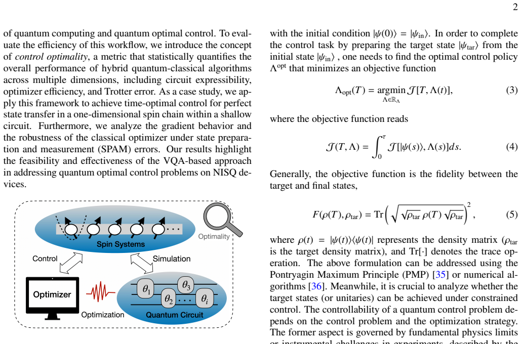
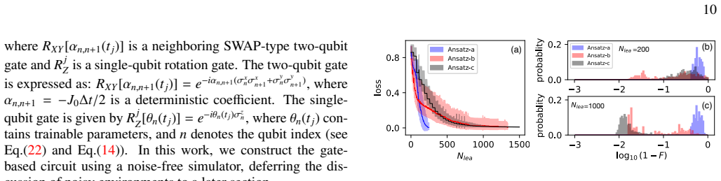
The central machinery is the Trotterized Hamiltonian-variational circuit U_HVA = ∏_{l=1}^{N_t} [U_0 ⊗_n R_z(θ_{n,l})], where U_0 = exp(−i J_0(σ_n^x σ_{n+1}^x + σ_n^y σ_{n+1}^y)T/N_t) is a fixed XY-exchange layer and R_z(θ_{n,l}) are trainable single-qubit rotations whose angles are mapped from control fields through θ_{γ,j}=f[λ_γ(t_j),n]. The three ansatze differ in how correlated these angles are: Ansatz-a uses one moving harmonic-trap center, Ansatz-b adds a time-dependent trap strength, and Ansatz-c uses N independent uncorrelated fields. The performance yardstick is control optimality, defined as the 1-Wasserstein distance W_1[P_lea(x), P_ref(x)] between the cumulative distribution of optimized log-infidelities x=log10(1−F) and a reference distribution concentrated at the fidelity threshold, with the normalized value W_1/ε lying in [0,1] and equaling 0 only when every optimization lands at the conditional optimum.
What would settle it
Run a dense numerical optimal-control search (for example, GRAPE or Krotov) over the same Ansatz-c control fields for N=6, J0=1, and find the smallest T at which fidelity 0.999 is attainable; independently compute the Mandelstam-Tamm time-averaged energy-dispersion bound along that optimal trajectory. If the true minimal T is larger than T≈2.52, or if the quoted QSL bound exceeds T≈2.52, then the paper's near-speed-limit claim is falsified.
Extended reading notes
Core claim
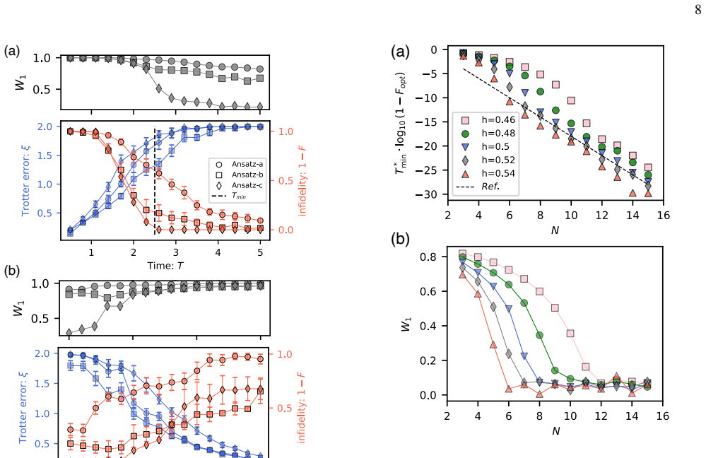
The discovery, stated on the paper's own terms, is that the variational quantum algorithm attains near-time-optimal perfect state transfer in a six-qubit XX chain at total time T≈2.52 with fidelity F>Fc=0.999, using the uncorrelated Ansatz-c whose trainable parameters are N independent z-rotation fields B2(t)={θ_n(t)}, with only Nt=N Trotter steps. The controlling estimate is Eq. (29), T_min=(N−1)/(2J0), which the paper treats as the speed limit for this setup; the same section also quotes the Mandelstam-Tamm expression τ_QSL=(N−1)π/(4J0). The paper further claims that its new control optimality metric, the normalized W1 distance between the empirical log-infidelity CDF and a reference delta/step distribution, is a more consistent predictor of VQA performance than the DKL expressibility metric, because W1 captures both the quantum circuit's expressibility and the classical optimizer's effectiveness, including cases where larger Trotter steps worsen optimization despite reducing Trotter error.
Load-bearing premise
The load-bearing premise is that T_min=(N−1)/(2J0) is the actual minimum time for perfect state transfer in the XX spin chain of Eq. (22), since the paper uses this value as the benchmark that its numerically found T≈2.52 approaches; the paper cites this formula but does not derive it for its own Hamiltonian and control set.
Editorial extensions
If this is right
- If the central claim is right, time-optimal control of a many-body spin chain does not require deep or highly correlated circuits: a shallow circuit with Nt=N Trotter steps suffices, and larger systems (N>9) remain within the tight time limit h≤0.5 with infidelity around 10^{-4}.
- Control optimality, unlike expressibility, can be used as a practical benchmarking number for hybrid workflows: it separates setups that only look expressive from setups whose optimizations actually land at the target fidelity.
- The observed gradient-variance scaling O(2^{-N}) instead of O(2^{-2N}) means that for these correlated, deterministic-layer circuits the barren-plateau problem is milder than for random 2-design ansatze, improving trainability at fixed circuit depth.
- Below the minimum time, the gradient variance decays as O(T^{2N}), so the speed limit itself shows up as a trainability limit: when there is not enough time to control the system, the optimizer's signal vanishes.
- The metric's definition for arbitrary cost functions means it can be extended to other hybrid algorithms and to noisy devices, where it should be computed from the same sampled fidelity outcomes without requiring convergence of the cost.
Reading between the lines
- Editorial extension: the strength of the speed-limit claim depends on Eq. (29) being the correct lower bound for this Hamiltonian; the Mandelstam-Tamm expression quoted in the same section gives a larger value for N=6, so the paper's 'closely approaching the quantum speed limit' should be read as approaching Eq. (29), not necessarily the tightest bound.
- As an extension, control optimality could be used online as a stopping criterion or ansatz-selection rule, since its sensitivity to the learning budget N_lea means it can detect when additional optimization effort no longer improves the distribution of outcomes.
- A neighboring problem worth checking is whether the same W1 metric orders quantum machine learning or closed-loop control tasks correctly, since expressibility is not a well-defined comparator there but W1 is.
- A natural test on hardware is to compute the W1 distance from repeated runs on a real device with finite shot noise and compare it with the noiseless simulator value; the paper's SPAM-error results predict a systematic shift of the apparent optimal time, which could be measured directly.
Editorial analysis
A structured set of objections, weighed in public.
Referee Report
Summary. The paper proposes a hybrid quantum-classical framework for quantum optimal control, in which a Trotterized circuit with trainable control parameters plays the role of a control policy and a classical optimizer minimizes the infidelity. The authors introduce a 'control optimality' metric based on the W1 Wasserstein distance between the distribution of optimized fidelities and a reference distribution at a fidelity threshold Fc. They apply this setup to perfect state transfer (PST) in a one-dimensional spin chain with three ansatz variants (Ansatz-a, -b, -c) and report that the uncorrelated Ansatz-c achieves fidelity above 0.999 at total time T≈2.52 for N=6, which they claim approaches the analytic minimum time Tmin=(N−1)/(2J0). They also study gradient-variance scaling and robustness to SPAM errors under depolarizing noise. The central claims are (i) the W1-based optimality metric tracks practical VQA performance better than the DKL expressibility metric, and (ii) a VQA with a shallow circuit (Nt=N) can solve time-optimal PST near the quantum speed limit.
Significance. If the claims are correct, the paper makes a useful conceptual contribution by introducing a workflow-level metric that jointly captures quantum and classical aspects of hybrid optimization, rather than only circuit expressibility or Trotter error. The numerical studies are internally consistent with the stated definitions, and the ranking of ansatze (Ansatz-c best, Ansatz-a worst) is supported by the reported W1 and fidelity data. The authors also provide openly available code. The most striking quantitative claim—that a VQA reaches a PST time close to the minimum time—is, however, not yet supported because of an inconsistency in the speed-limit formulas used as the benchmark. The gradient-scaling result (O(2−N) rather than O(2−2N)) is interesting but would benefit from a more explicit explanation of why the ansatz is not a 2-design.
major comments (4)
- [Section IV.B and Eq. (29)] The manuscript states τ_QSL ≤ T_min and quotes τ_QSL=(N−1)π/(4J0) immediately before Eq. (29), which gives Tmin=(N−1)/(2J0). For N=6 these are 3.93 and 2.50, respectively, so the quoted inequality is false. The reported value T≈2.52 is compared only to the smaller value 2.50, and the abstract's claim of 'closely approaching the quantum speed limit' is therefore ambiguous or unsupported if 3.93 is the operative bound. Please reconcile the two expressions, or state precisely which lower bound applies to the model of Eq. (22) and justify that choice.
- [Eqs. (9), (25), and Appendix A] The Trotter time step is defined as Δt=T/(Nt−1) in Eq. (9) and in Appendix A, but Eq. (25) uses T/Nt in the exponent of the static unitary layer. With Nt=N=6 and the reported T=2.52, the first convention gives a physical evolution time of 6×2.52/5=3.02, which is 20% larger than the quoted T. The manuscript does not state which convention the simulations use, so the reported 'minimum time' is not well-defined. Please specify the convention and recompute the reported T values accordingly.
- [Section IV.B, benchmark derivation] Eq. (29), Tmin=(N−1)/(2J0), is quoted from Refs. [55,70,71] but is not derived for the Hamiltonian in Eq. (22) with the unbounded z-control fields of Eq. (24). Because this formula is the benchmark against which the claim T≈2.52 is judged, the authors should provide a derivation or a reference that establishes the lower bound for this specific control family and interaction model; otherwise the speed-limit comparison lacks a rigorous footing.
- [Section V, 'better than conventional methods'] The conclusion states that the VQA 'performing even better than previous conventional methods (h<0.5 in Fig. 5)'. However, Fig. 5 does not contain any comparison to conventional methods; the parameter h is merely a scaling factor that sets the total simulation time in the VQA runs. Please add a direct comparison with, e.g., the methods of Refs. [60–62], or reformulate the claim so that it does not imply a benchmark comparison that is not shown.
minor comments (4)
- [Abstract and Introduction] There is a typo in the introduction ('we fisrt provide') and in Section III.A ('on shall calculate'); the paper would benefit from a careful proofreading pass.
- [Fig. 6(b) caption] The caption states Nt=2N, while the text in Section IV.B and Fig. 6(a) use Nt=N; please make the circuit-depth convention consistent across the figure and the text.
- [Section III.B, Eq. (17)] The notation for the Iverson bracket and the reference distribution Pref(F) is somewhat informal; a cleaner definition with the domain of F would improve readability.
- [Fig. 3(d)] The label 'Dkl' should be 'DKL' for consistency with Eq. (15), and the caption of Fig. 4 could clarify which panel shows the W1 distance (the upper panel is not explicitly labeled).
Circularity Check
Control-optimality superiority claim is definitional, but PST numerics and gradient scalings are independently computed; speed-limit inconsistency is a correctness issue, not circularity.
-
self definitional
[Section IV.A (The maximum-fidelity control), final paragraph after Fig. 3; cf. Eqs. (18)-(19) and (21).]
"Then we can conclude that to evaluate the overall performance of a VQA, one should estimate control optimality rather than expressibility for the following reasons:W1 reflects both the expressibility of the quantum circuit and the performance of the classical optimizer, whereas DKL only captures the former."
By Eqs. (18)-(19), Plea(F;Nlea) is the learning fidelity distribution accumulated during optimization, and Optim is the W1 distance from Plea to the reference optimal delta distribution. Therefore the claim that W1 'reflects the performance of the classical optimizer' is a restatement of the definition: W1 is a functional of exactly the achieved-fidelity outcomes whose quality it is used to rank. The empirical observation that W1 orders Ansatz-a/b/c consistently with infidelity is not an independent confirmation of the metric but an identity up to the chosen reference distribution. The PST time-optimal result and the gradient scaling laws are separate computed/fitted results and do not reduce this way, so the circularity is partial.
full rationale
The central time-optimal PST claim (T≈2.52 close to Eq. (29)) is a numerical result obtained by optimizing circuit parameters; it is not derived from the W1 metric, and Eq. (29) is an external benchmark rather than a fitted input. The gradient scalings O(2^-N) and O(T^{2N}) are empirical scalings fitted to the data, not predictions presented as derived. The main circularity is the metric-superiority claim: control optimality is defined as the W1 distance between the optimizer-produced fidelity distribution and an ideal reference, so showing that it tracks optimizer performance is largely tautological. Self-citations such as [13], [54], and [75] are not load-bearing for the central derivation. The internal inconsistency between tau_QSL=(N-1)pi/(4J0), Tmin=(N-1)/(2J0), and the two Trotter-time conventions is an important correctness and consistency concern, but it is not a circularity, and it does not enter the circularity score.
Assumptions & free parameters
free parameters (3)
- Fidelity threshold Fc =
0.999
- Time-scaling factor h in Eq. (30) =
0.46, 0.48, 0.5, 0.52, 0.54
- Gradient scaling exponent 2N in Eq. (31) =
2N
assumptions (5)
- standard math Trotter-Suzuki first-order product formula approximates the continuous propagator and the Trotter error is measured by Eq. (11).
- standard math The single-excitation subspace is sufficient because total z-magnetization is conserved ([HXXZ, sum sigma_z] = 0).
- ad hoc to paper W1 distance between sampled fidelity distributions is a meaningful measure of overall hybrid workflow performance.
- domain assumption Eq. (29), Tmin=(N-1)/(2J0), is the valid lower bound for the PST problem and can serve as the speed-limit benchmark.
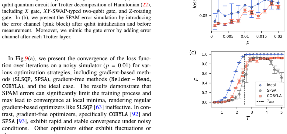
- domain assumption The reported fidelities are achieved by the classical optimizers (SLSQP, COBYLA, SPSA) with the exact or finite-shot cost model, and these results transfer to a real NISQ device.
Cite this review
Pith. "Pith review of Optimal Control by Variational Quantum Algorithms." pith.science (2026). https://pith.science/paper/7WTY6OI6
@misc{pith2026250523373,
  author       = {Pith},
  title        = {Pith review of: Optimal Control by Variational Quantum Algorithms},
  year         = {2026},
  howpublished = {\url{https://pith.science/paper/7WTY6OI6}},
  note         = {Machine review of arXiv:2505.23373}
}
read the original abstract
Hybrid quantum-classical algorithms hold great promise for solving quantum control problems on near-term quantum computers. In this work, we employ the hybrid framework that integrates digital quantum simulation with classical optimization to achieve optimal engineering of quantum many-body systems. To evaluate the overall performance of this method, we introduce a general metric termed control optimality, which accounts for constraints on both classical and quantum components. As a concrete example, we investigate the time-optimal control for perfect state transfer in a one-dimensional spin model using the variational quantum algorithm, closely approaching the quantum speed limit. Moreover, we discuss the emergent gradient behavior and error robustness, demonstrating the feasibility of applying hybrid quantum algorithms to solve quantum optimal control problems. These results establish a systematic framework for hybrid algorithms to address quantum control problems on near-term quantum platforms.
Figures


Figures from the paper (5 more)


Reference graph
Works this paper leans on
-
[1]
Initialization: We firstly initialize the control policy Λ(0) = Λ 0 and prepare the qubit-register with state ρ(0) =ρin
-
[2]
The circuit consists of alternating layers of gates, repre- senting the time evolution under various control Hamil- tonians Hγ with control-related anglesθ(λγ, t j)
Circuit Construction: Secondly, we construct the PQC U(θ) formed by DQS of driving propagator (Eq.(2) ) U(θ)≡ NtY j=1 ΓY γ=1 exp −iHγθ(λγ, t j)∆t V j, (9) V j represents the evolution under the static Hamiltonian term and ∆t = T/(Nt− 1) is the discrete time interval. The circuit consists of alternating layers of gates, repre- senting the time evolution un...
-
[3]
The optimization target is: θopt = argmin θ∈R 1− F(ρ(T),ρ tar) , (10) where F(·) is defined in Eq.(5) and the final state reads ρ(T) = U(θ)ρ0U(θ)†
Optimization: Thirdly, a classical optimizer updates the parameters θ∈ R by minimizing the infidelity be- tween the final state ρ(T) and the target state ρtar. The optimization target is: θopt = argmin θ∈R 1− F(ρ(T),ρ tar) , (10) where F(·) is defined in Eq.(5) and the final state reads ρ(T) = U(θ)ρ0U(θ)†. In this paper, the Trotter errors for a total tim...
-
[4]
Feynman, Optics news 11, 11 (1985)
R. Feynman, Optics news 11, 11 (1985)
1985
-
[5]
A. J. Daley, I. Bloch, C. Kokail, S. Flannigan, N. Pearson, M. Troyer, and P. Zoller, Nature607, 667 (2022)
2022
-
[6]
Katabarwa, K
A. Katabarwa, K. Gratsea, A. Caesura, and P. D. Johnson, PRX Quantum 5, 020101 (2024)
2024
-
[7]
Bauer, S
B. Bauer, S. Bravyi, M. Motta, and G. K.-L. Chan, Chemical 12 Reviews 120, 12685 (2020)
2020
-
[8]
Portmann and R
C. Portmann and R. Renner, Rev. Mod. Phys. 94, 025008 (2022)
2022
Show all 95 references
-
[9]
Farhi, J
E. Farhi, J. Goldstone, and S. Gutmann, A quantum approxi- mate optimization algorithm (2014), arXiv:1411.4028 [quant- ph]
2014 arXiv
-
[11]
Cerezo, A
M. Cerezo, A. Arrasmith, R. Babbush, S. C. Benjamin, S. Endo, K. Fujii, J. R. McClean, K. Mitarai, X. Yuan, L. Cincio, et al., Nature Reviews Physics 3, 625 (2021)
2021
-
[12]
A. B. Magann, C. Arenz, M. D. Grace, T.-S. Ho, R. L. Kosut, J. R. McClean, H. A. Rabitz, and M. Sarovar, PRX Quantum2, 010101 (2021)
2021
-
[13]
de Keijzer, O
R. de Keijzer, O. Tse, and S. Kokkelmans, Quantum 7, 908 (2023)
2023
-
[14]
Choquette, A
A. Choquette, A. Di Paolo, P. K. Barkoutsos, D. S ´en´echal, I. Tavernelli, and A. Blais, Phys. Rev. Res.3, 023092 (2021)
2021
-
[15]
J. Li, X. Yang, X. Peng, and C.-P. Sun, Phys. Rev. Lett. 118, 150503 (2017)
2017
-
[16]
Huang, Y
T. Huang, Y . Ding, L. Dupays, Y . Ban, M.-H. Yung, A. del Campo, and X. Chen, Phys. Rev. Res. 5, 023173 (2023)
2023
-
[17]
P. J. Ollitrault, G. Mazzola, and I. Tavernelli, Phys. Rev. Lett. 125, 260511 (2020)
2020
-
[18]
A. B. Magann, M. D. Grace, H. A. Rabitz, and M. Sarovar, Phys. Rev. Res. 3, 023165 (2021)
2021
-
[19]
N. N. Hegade, K. Paul, Y . Ding, M. Sanz, F. Albarr ´an- Arriagada, E. Solano, and X. Chen, Phys. Rev. Appl. 15, 024038 (2021)
2021
-
[20]
Or ´us, Nature Reviews Physics 1, 538 (2019)
R. Or ´us, Nature Reviews Physics 1, 538 (2019)
2019
-
[21]
Suzuki, Communications in Mathematical Physics 51, 183 (1976)
M. Suzuki, Communications in Mathematical Physics 51, 183 (1976)
1976
-
[22]
Preskill, Quantum 2, 79 (2018)
J. Preskill, Quantum 2, 79 (2018)
2018
-
[23]
Y . Kim, C. J. Wood, T. J. Yoder, S. T. Merkel, J. M. Gambetta, K. Temme, and A. Kandala, Nature Physics 19, 752 (2023)
2023
-
[24]
Smith, M
A. Smith, M. Kim, F. Pollmann, and J. Knolle, npj Quantum Information 5, 106 (2019)
2019
-
[25]
Fauseweh, Nature Communications 15, 2123 (2024)
B. Fauseweh, Nature Communications 15, 2123 (2024)
2024
-
[26]
Torlai and R
G. Torlai and R. G. Melko, Annual Review of Condensed Mat- ter Physics 11, 325 (2020)
2020
-
[27]
J. R. McClean, S. Boixo, V . N. Smelyanskiy, R. Babbush, and H. Neven, Nature communications 9, 1 (2018)
2018
-
[28]
S. Wang, E. Fontana, M. Cerezo, K. Sharma, A. Sone, L. Cin- cio, and P. J. Coles, Nature communications 12, 1 (2021)
2021
-
[29]
Cerezo, A
M. Cerezo, A. Sone, T. V olkoff, L. Cincio, and P. J. Coles, Na- ture communications 12, 1 (2021)
2021
-
[30]
S. Sim, P. D. Johnson, and A. Aspuru-Guzik, Advanced Quan- tum Technologies 2, 1900070 (2019)
2019
-
[31]
Nakaji and N
K. Nakaji and N. Yamamoto, Quantum 5, 434 (2021)
2021
-
[32]
Yi, Phys
C. Yi, Phys. Rev. A 104, 052603 (2021)
2021
-
[33]
Layden, Phys
D. Layden, Phys. Rev. Lett. 128, 210501 (2022)
2022
-
[34]
L. K. Kovalsky, F. A. Calderon-Vargas, M. D. Grace, A. B. Ma- gann, J. B. Larsen, A. D. Baczewski, and M. Sarovar, Phys. Rev. Lett. 131, 060602 (2023)
2023
-
[35]
Zhang, J
Z.-J. Zhang, J. Sun, X. Yuan, and M.-H. Yung, Phys. Rev. Lett. 130, 040601 (2023)
2023
-
[36]
H. Zhao, M. Bukov, M. Heyl, and R. Moessner, PRX Quantum 4, 030319 (2023)
2023
-
[37]
Wurtz and P
J. Wurtz and P. J. Love, Quantum 6, 635 (2022)
2022
-
[38]
Boscain, M
U. Boscain, M. Sigalotti, and D. Sugny, PRX Quantum 2, 030203 (2021)
2021
-
[39]
M. M. M ¨uller, R. S. Said, F. Jelezko, T. Calarco, and S. Mon- tangero, Reports on progress in physics 85, 076001 (2022)
2022
-
[40]
Leone, S
L. Leone, S. F. Oliviero, L. Cincio, and M. Cerezo, Quantum 8, 1395 (2024)
2024
-
[41]
Park and N
C.-Y . Park and N. Killoran, Quantum8, 1239 (2024)
2024
-
[42]
Wecker, M
D. Wecker, M. B. Hastings, and M. Troyer, Phys. Rev. A 92, 042303 (2015)
2015
-
[43]
A. M. Childs, Y . Su, M. C. Tran, N. Wiebe, and S. Zhu, Phys. Rev. X 11, 011020 (2021)
2021
-
[44]
Mitarai, M
K. Mitarai, M. Negoro, M. Kitagawa, and K. Fujii, Phys. Rev. A 98, 032309 (2018)
2018
-
[45]
Schuld, V
M. Schuld, V . Bergholm, C. Gogolin, J. Izaac, and N. Killoran, Phys. Rev. A 99, 032331 (2019)
2019
-
[46]
R. P. Feynman, in Feynman and computation (CRC Press,
-
[47]
Hunter-Jones, Unitary designs from statistical mechanics in random quantum circuits (2019), arXiv:1905.12053 [quant-ph]
N. Hunter-Jones, Unitary designs from statistical mechanics in random quantum circuits (2019), arXiv:1905.12053 [quant-ph]
2019 arXiv
-
[48]
Mezzadri, How to generate random matrices from the classi- cal compact groups (2007), arXiv:math-ph/0609050 [math-ph]
F. Mezzadri, How to generate random matrices from the classi- cal compact groups (2007), arXiv:math-ph/0609050 [math-ph]
2007 arXiv
-
[49]
Heyraud, Z
V . Heyraud, Z. Li, K. Donatella, A. Le Boit´e, and C. Ciuti, PRX Quantum 4, 040335 (2023)
2023
-
[50]
Holmes, K
Z. Holmes, K. Sharma, M. Cerezo, and P. J. Coles, PRX Quan- tum 3, 010313 (2022)
2022
-
[51]
Du, M.-H
Y . Du, M.-H. Hsieh, T. Liu, S. You, and D. Tao, PRX Quantum 2, 040337 (2021)
2021
-
[52]
E. T. Jaynes, Phys. Rev. 106, 620 (1957)
1957
-
[53]
A. J. Majda and B. Gershgorin, Proceedings of the National Academy of Sciences 108, 10044 (2011)
2011
-
[54]
V . M. Panaretos and Y . Zemel, Annual review of statistics and its application 6, 405 (2019)
2019
-
[55]
Demiralp and H
M. Demiralp and H. Rabitz, Phys. Rev. A 57, 2420 (1998)
1998
-
[56]
H. A. Rabitz, M. M. Hsieh, and C. M. Rosenthal, Science 303, 1998 (2004)
2004
-
[57]
Huang, A
T. Huang, A. Gaikwad, I. Moskalenko, A. Aggarwal, T. Abad, M. Kuzmanovic, Y .-H. Chang, O. Stanisavljevic, E. Hogedal, C. Warren, I. Ahmad, J. Bizn ´arov´a, A. Osman, M. Dahiya, M. Rommel, A. F. Rousari, A. Nylander, L. Chen, J. Bylan- der, G. S. Paraoanu, A. F. Kockum, and G....
2025
-
[58]
Yung, Phys
M.-H. Yung, Phys. Rev. A 74, 030303 (2006)
2006
-
[59]
R. J. Chapman, M. Santandrea, Z. Huang, G. Corrielli, A. Crespi, M.-H. Yung, R. Osellame, and A. Peruzzo, Nature communications 7, 11339 (2016)
2016
-
[60]
Balachandran and J
V . Balachandran and J. Gong, Phys. Rev. A77, 012303 (2008)
2008
-
[61]
M. I. Makin, J. H. Cole, C. D. Hill, and A. D. Greentree, Phys. Rev. Lett. 108, 017207 (2012)
2012
-
[62]
M. H. Ahmed and A. D. Greentree, Phys. Rev. A 91, 022306 (2015)
2015
-
[63]
Caneva, M
T. Caneva, M. Murphy, T. Calarco, R. Fazio, S. Montangero, V . Giovannetti, and G. E. Santoro, Phys. Rev. Lett.103, 240501 (2009)
2009
-
[64]
Murphy, S
M. Murphy, S. Montangero, V . Giovannetti, and T. Calarco, Phys. Rev. A 82, 022318 (2010)
2010
-
[65]
Zhang, Z.-W
X.-M. Zhang, Z.-W. Cui, X. Wang, and M.-H. Yung, Phys. Rev. A 97, 052333 (2018)
2018
-
[66]
P. T. Boggs and J. W. Tolle, Acta numerica4, 1 (1995)
1995
-
[67]
Mandelstam and I
L. Mandelstam and I. Tamm, J. Phys. USSR 9, 249 (1945)
1945
-
[68]
Anandan and Y
J. Anandan and Y . Aharonov, Phys. Rev. Lett.65, 1697 (1990)
1990
-
[69]
Uhlmann, Physics Letters A 161, 329 (1992)
A. Uhlmann, Physics Letters A 161, 329 (1992)
1992
-
[70]
Margolus and L
N. Margolus and L. B. Levitin, Physica D: Nonlinear Phenom- ena 120, 188 (1998)
1998
-
[71]
De ffner and E
S. De ffner and E. Lutz, Journal of Physics A: Mathematical and Theoretical 46, 335302 (2013)
2013
-
[72]
De ffner and S
S. De ffner and S. Campbell, Journal of Physics A: Mathemati- cal and Theoretical 50, 453001 (2017)
2017
-
[73]
A. Kay, W. Xie, and C. Tamon, A note on the speed of perfect 13 state transfer (2022), arXiv:1609.01854 [quant-ph]
2022 arXiv
-
[74]
Ashhab, P
S. Ashhab, P. C. de Groot, and F. Nori, Phys. Rev. A85, 052327 (2012)
2012
-
[75]
Christandl and R
M. Christandl and R. Renner, Phys. Rev. Lett. 109, 120403 (2012)
2012
-
[76]
Proctor, S
T. Proctor, S. Seritan, K. Rudinger, E. Nielsen, R. Blume- Kohout, and K. Young, Phys. Rev. Lett.129, 150502 (2022)
2022
-
[77]
A. M. Palmieri, E. Kovlakov, F. Bianchi, D. Yudin, S. Straupe, J. D. Biamonte, and S. Kulik, npj Quantum Information 6, 20 (2020)
2020
-
[78]
Huang, Y
T. Huang, Y . Ban, E. Y . Sherman, and X. Chen, Phys. Rev. Appl. 17, 024040 (2022)
2022
-
[79]
Y . Wang, Y . Ding, F. A. C´ardenas-L´opez, and X. Chen, Phys. Rev. Appl. 22, 024009 (2024)
2024
-
[80]
B. Li, S. Ahmed, S. Saraogi, N. Lambert, F. Nori, A. Pitchford, and N. Shammah, Quantum 6, 630 (2022)
2022
-
[81]
Cerezo, G
M. Cerezo, G. Verdon, H.-Y . Huang, L. Cincio, and P. J. Coles, Nature computational science 2, 567 (2022)
2022
-
[82]
Kelly, R
J. Kelly, R. Barends, B. Campbell, Y . Chen, Z. Chen, B. Chiaro, A. Dunsworth, A. G. Fowler, I.-C. Hoi, E. Jeffrey, A. Megrant, J. Mutus, C. Neill, P. J. J. O’Malley, C. Quintana, P. Roushan, D. Sank, A. Vainsencher, J. Wenner, T. C. White, A. N. Cleland, and J. M. Martinis, P...
2014
-
[83]
Doria, T
P. Doria, T. Calarco, and S. Montangero, Phys. Rev. Lett. 106, 190501 (2011)
2011
-
[84]
Kiely and S
A. Kiely and S. Campbell, New Journal of Physics 23, 033033 (2021)
2021
-
[85]
Coopmans, S
L. Coopmans, S. Campbell, G. De Chiara, and A. Kiely, Phys. Rev. Res. 4, 043138 (2022)
2022
-
[86]
Safavi-Naini, R
A. Safavi-Naini, R. J. Lewis-Swan, J. G. Bohnet, M. G ¨arttner, K. A. Gilmore, J. E. Jordan, J. Cohn, J. K. Freericks, A. M. Rey, and J. J. Bollinger, Phys. Rev. Lett.121, 040503 (2018)
2018
-
[87]
Richerme, C
P. Richerme, C. Senko, J. Smith, A. Lee, S. Korenblit, and C. Monroe, Phys. Rev. A 88, 012334 (2013)
2013
-
[88]
X. Xu, J. Cui, Z. Cui, R. He, Q. Li, X. Li, Y . Lin, J. Liu, W. Liu, J. Lu,et al., Mindspore quantum: A user-friendly, high- performance, and ai-compatible quantum computing frame- work (2024), arXiv:2406.17248 [quant-ph]
2024 arXiv
-
[89]
D. A. Rower, L. Ding, H. Zhang, M. Hays, J. An, P. M. Harring- ton, I. T. Rosen, J. M. Gertler, T. M. Hazard, B. M. Niedzielski, M. E. Schwartz, S. Gustavsson, K. Serniak, J. A. Grover, and W. D. Oliver, PRX Quantum5, 040342 (2024)
2024
-
[90]
e. a. Barends, R, Phys. Rev. Lett. 123, 210501 (2019)
2019
-
[91]
B. e. a. Foxen (Google AI Quantum), Phys. Rev. Lett. 125, 120504 (2020)
2020
-
[92]
U. L. Heras, A. Mezzacapo, L. Lamata, S. Filipp, A. Wallra ff, and E. Solano, Phys. Rev. Lett. 112, 200501 (2014)
2014
-
[93]
X. Yang, J. Chu, Z. Guo, W. Huang, Y . Liang, J. Liu, J. Qiu, X. Sun, Z. Tao, J. Zhang, J. Zhang, L. Zhang, Y . Zhou, W. Guo, L. Hu, J. Jiang, Y . Liu, X. Linpeng, T. Chen, Y . Chen, J. Niu, S. Liu, Y . Zhong, and D. Yu, Phys. Rev. Lett. 133, 170601 (2024)
2024
-
[94]
M. A. Nielsen and I. Chuang, Quantum computation and quantum information (Ameri- can Association of Physics Teachers, 2002)
2002
-
[95]
M. J. Powell, Acta numerica 7, 287 (1998)
1998
-
[96]
J. C. Spall, Johns Hopkins apl technical digest 19, 482 (1998)
1998
Reviewed August 7, 2026 · model on record in the stance chip above.
Discussion (0). Sign in to comment.