REVIEW 3 major objections 5 minor 27 references
Instance-Optimality for Private KL Distribution Estimation
T0 review · 3 major / 5 minor · reviewed 2026-08-07 · deepseek-v4-flash
Pith's one-line read The paper establishes that private KL distribution estimation can be instance-optimal: a differentially private 'sampling twice' Good-Turing estimator achieves per-instance KL error within a constant factor of the per-instance minimax…
desk verdict First DP KL minimax rates and a clever sampling-twice estimator, but the printed neighborhood definition contradicts the proofs; the headline instance-optimality theorem needs a fix before it is established. read the letter →
The pith
A machine-rendered reading of the paper's core claim, the machinery that carries it, and where it could break.
The reading
What carries the argument
Two mechanisms carry the argument. First, the 'sampling twice' estimator: split the Poisson sample into two halves, use one half to decide which symbols have small counts, use the other half to estimate the combined mass of those symbols, and truncate individual noisy counts at a floor $\max\{\cdot, 1/\min\{\varepsilon,1\}\}$. This reduces the sensitivity to adjacent datasets to one, which is what makes a Good-Turing-style bias correction privatizable. Second, the lower-bound analysis is driven by a generalized Assouad's method (Theorems A.3 and A.4) that applies to any decomposable statistical distance; KL is decomposable in the sense that $\mathrm{KL}(p,q) \ge \sum_j p(B_j)\,\mathrm{KL}(p|_{B_j}, q|_{B_j})$ over disjoint symbol blocks. For the DP algorithm, a calibrated threshold $\tau = 4\ln d$ (equivalently neighborhood size $t=24\ln d$) balances false positives (small-probability symbols treated as large) against false negatives (large-probability symbols treated as small), which is the quantitative core of the instance-optimality proof.
What would settle it
Run Algorithm 2 on a power-law distribution $p_i \propto i^{-\beta}$ with $d=50{,}000$, $n=10^4$, and $\varepsilon=1$; estimate $\mathbb{E}[\mathrm{KL}(p,A(x))]$ by repeated Poisson sampling and compare it with $\mathrm{lower}(p,n,\mathcal{N}^+ \cup \mathcal{N}_{\le 24\ln d/(n\varepsilon)})$ evaluated from the formulas in the paper. If the empirical error is more than a large constant factor above this bound, or if the ratio grows with $d$, the claimed constant-factor instance-optimality fails.
Extended reading notes
Core claim
Central claim: under the additive neighborhoods $\mathcal{N}^+(p) = \{q: |q_i-p_i| \le \min\{t/n,\sqrt{p_i/n}\}, \sum_{i:p_i\le t/n} q_i \le \max\{t/n,\sum p_i\}\}$ (and the privacy-scaled $\mathcal{N}_{\le t/(n\varepsilon)}$ version), per-instance KL error is tightly characterized. Concretely, Algorithm 2 is $\varepsilon$-DP and satisfies $\mathbb{E}_{x\sim \mathrm{Poi}(np)}[\mathrm{KL}(p,A(x))] \le O(\mathrm{lower}(p,n,\mathcal{N}^+ \cup \mathcal{N}_{\le 24\ln d/(n\varepsilon)}))$, i.e. it is competitive with any estimator that knows the truth lies in that small additive ball; Algorithm 1 achieves the non-private analogue. The lower bounds are proved for any estimator via a generalized Assouad's method for decomposable statistical distances, exploiting that KL divergence is decomposable. The paper further shows this neighborhood scale is necessary up to constants: no $(\varepsilon,\delta)$-DP estimator can be instance-optimal with respect to neighborhoods of size $\gamma \ln d/(n\varepsilon)$ for $\gamma=o(1)$.
Load-bearing premise
The load-bearing premise is that additive perturbation of each symbol's probability—by $\min\{t/n,\sqrt{p_i/n}\}$ in the non-private case and $t/(n\varepsilon)$ under privacy—is the right way to measure how hard a distribution is; if the genuinely hard alternatives require changing symbol identities or reordering, the instance-optimality guarantees would be measuring the wrong kind of difficulty.
Editorial extensions
If this is right
- For each fixed $p$, the DP algorithm's expected KL error is bounded by a constant times $\mathrm{lower}(p,n,\mathcal{N}^+\cup\mathcal{N}_{\le t/(n\varepsilon)})$; distributions with a few heavy symbols or small combined mass on rare symbols are therefore estimated far below the worst-case $\ln(1+d/n)$ rate.
- Privacy is essentially free for symbols with large $p_i$: their contribution to the private bound is $1/(n^2\varepsilon^2 p_i)$, smaller than the non-private $1/n$ term, so the DP penalty concentrates on rare symbols.
- The neighborhood size $\Theta(\ln d/(n\varepsilon))$ is necessary for worst-case DP instance-optimality: for any $\gamma=o(1)$, no DP estimator can match a baseline that knows a neighborhood of size $\gamma \ln d/(n\varepsilon)$.
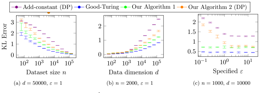
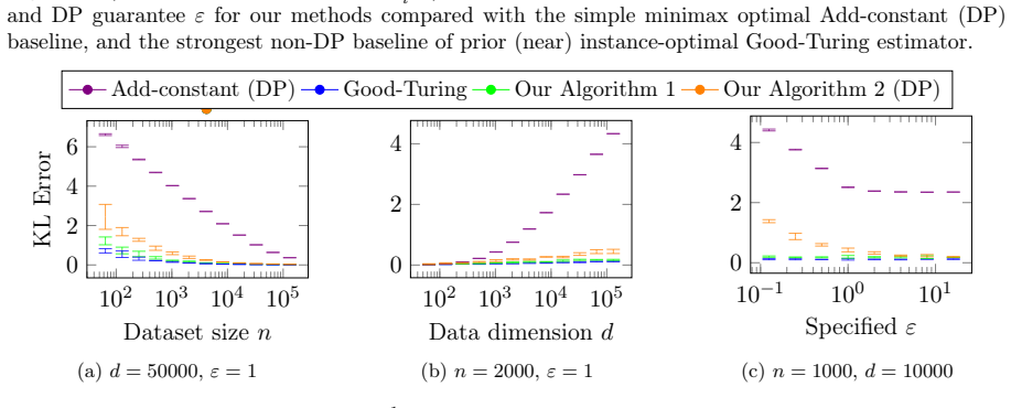
- The non-private 'sampling twice' algorithm matches the per-instance lower bound up to constants under additive neighborhoods, and in experiments it is competitive with the prior Good-Turing baseline while being easier to privatize.
- The experiments show the DP algorithm outperforming the minimax-optimal add-constant DP baseline on power-law and real token distributions, which the instance-optimality guarantee predicts.
Reading between the lines
- The sensitivity reduction from splitting the sample is not KL-specific, so a similar 'sampling twice' construction could plausibly yield private instance-optimal estimators for other decomposable losses such as total variation or $\ell^2$ error under the same additive-neighborhood framework.
- The threshold $\tau=4\ln d$ acts as an automatic, privacy-aware smoothing schedule: symbols whose noisy counts fall below threshold are pooled and their mass is estimated from fresh data; this suggests a testable recipe for language-model smoothing against fixed add-constant baselines.
- The necessity theorem draws a sharp boundary: any stronger instance-level guarantee for private KL estimation would have to change what the hypothetical knowledgeable estimator is allowed to know (a different neighborhood definition), not merely tighten constants.
Editorial analysis
A structured set of objections, weighed in public.
Referee Report
Summary. The paper studies KL divergence estimation of discrete distributions under differential privacy. It first establishes minimax optimal rates for private KL estimation, showing that a Laplace-perturbed add-constant estimator is optimal up to constants. It then introduces additive local neighborhoods of a distribution, N+(p) and N≤t/(nε)(p), and proposes 'sampling-twice' Good-Turing-style estimators (Algorithm 1 non-private, Algorithm 2 private) that are claimed to be instance-optimal up to constant factors relative to these neighborhoods. The lower bounds use a generalized Assouad method for decomposable statistical distances, and the upper bounds analyze false-positive/false-negative errors under calibrated thresholding. Experiments on power-law and token distributions show improvement over the minimax add-constant baseline.
Significance. If the results hold as stated, this is a significant contribution: it appears to be the first tight minimax analysis of private KL distribution estimation, and the first instance-optimality guarantees for private KL estimation under a notion of local neighborhood. The proofs are parameter-free in the sense that the bounds are explicit functions of p, n, and ε, and the algorithms are concrete and reproducible from the pseudocode. The paper also correctly identifies limitations of permutation and multiplicative neighborhoods for KL loss. However, the central neighborhood definition N+ is printed inconsistently with the surrounding discussion and with the proofs in Appendix D, which is load-bearing for the instance-optimality claims; the paper should be revised to fix this definition and to reconcile the Algorithm 2 pseudocode with its analysis.
major comments (3)
- [Section 2, Eq. (4); Appendix D; Corollary G.7] The printed definition of N+(p) uses |qi-pi| ≤ min{t/n, sqrt(pi/n)}, but the prose immediately above it says that symbols with pi > t/n should allow the larger sqrt(pi/n) perturbation, and Appendix D defines Nstat (Eq. 137) and N<=t/n (Eq. 136) as sub-neighborhoods of N+. With the printed min, Nstat is not contained in N+: for pi > t^2/n the allowed perturbation is t/n, which is smaller than sqrt(pi/n), and for pi=0 the allowed perturbation is 0, so no distribution with positive mass on a zero-probability symbol lies in N+. Consequently the claim lower(p,n,N+) ≥ (1/2)lower(p,n,N<=t/n) + (1/2)lower(p,n,Nstat) is false under the printed definition. Concretely, for p=(1/3,2/3,0,...,0), the printed N+ has support only on {1,2}, so lower(p,n,N+) ≤ O(1/n), whereas Eq. (5) with L' containing zero-probability symbols claims Ω(ln(1+d)/n). Since Theorem G.6 and Corollary G.7 match Algorithm 2 against lower(p,n,N+ ∪ N≤t/(nε)), the central instance-optimality result is not established for the neighborhood as written. The intended definition appears to be max{t/n, sqrt(pi/n)} (or an equivalent two-regime definition), which is what the proofs and the surrounding discussion presuppose; the manuscript must correct Eq. (4) and re-verify the subsequent lower-bound decomposition.
- [Section 3.1, Algorithm 2] The pseudocode of Algorithm 2 is internally inconsistent. The truncation step defines \bar{x}_i for i in L and for i not in L, but the return statement uses \bar{x}'_i in both branches, and the normalizing constant is N = \tilde{c} + sum_{i notin L} \bar{x}_i, while the returned mass for i not in L is (1/N)\bar{x}'_i. As printed, \bar{x}'_i is undefined and the output is not a probability vector. The lemmas in Appendix G (e.g., Lemma G.3, Lemma G.4, Lemma G.5) and Theorem G.6 analyze the estimator in terms of \bar{x}_i, so the pseudocode does not match the analyzed estimator. The pseudocode should be rewritten consistently, presumably replacing \bar{x}'_i with \bar{x}_i in both branches and using a single normalization sum, and the DP sensitivity argument in Theorem G.6 should be rechecked with the corrected expression.
- [Appendix D, decomposition of lower(p,n,N+)] Even setting aside the min/max typo, the sentence 'their average is a lower bound ... because one can construct a distribution over hard instances, choosing the hard instance(s) in N<=t/n and Nstat with 1/2 probability respectively' is imprecise. The correct valid step is that for a union N = N1 ∪ N2, max_{q∈N} ≥ (1/2)max_{q∈N1} + (1/2)max_{q∈N2}, which implies the claimed inequality without constructing a mixture over hard instances. The paper should replace the vague averaging argument with this direct inequality, and should also state explicitly that the inclusion N1, N2 ⊆ N+ is required for the decomposition.
minor comments (5)
- [Appendix E, Corollary E.3] In the proof, the citation 'lower(p, n, Nstat) in Theorem F.2' is incorrect: Theorem F.2 is the DP lower bound for N≤t/(nε), while the relevant non-DP Nstat lower bound is Theorem D.4 in Appendix D. Please fix the cross-reference.
- [Section 3.1, Theorem G.9] In the proof of Theorem G.9, the text 'by ε = ln d / 2n' does not match the theorem statement's ε = ln(d)/(16n). With the stated value, the displayed bound still holds because 2γ ln d/(nε) + γ(ln d)^2/(nε) = 32γ ln d + 16γ ln d = 48γ ln d, so the factor is consistent after correcting the typo in the proof.
- [Section 2, Eq. (5)] The statement of the per-instance lower bound (5) says 'for any set L′', but in the matching results (e.g., Corollary G.7) the relevant quantity is the maximum over L′ of the displayed expression. Please clarify in the text that the instance-optimality matching uses sup_{L′⊆[d]} of the right-hand side.
- [Section 4] There is a typo in the experimental setup: 'MacOS intergrated CPU' should be 'MacOS integrated CPU'. Also, the figure captions reference 'Reddit Token Distribution Estimation' but do not describe error bars or the number of trials beyond the text; adding this to the captions would improve reproducibility.
- [Section 3.1, Algorithm 2 and Theorem G.6] The pseudocode sets τ = 4 ln d, but Theorem G.6 states a general bound without explicitly displaying τ; the proof uses τ = 4 ln d. Please make the dependence of the upper bound on τ explicit in the theorem statement, and state the final choice τ = 4 ln d there.
Circularity Check
No significant circularity; the upper/lower matching is self-contained. The Eq. (4) min/max inconsistency is a correctness issue, not a circularity issue.
full rationale
The derivation chain is not circular in the sense defined by the review rules. The instance-optimality benchmark lower(p,n,N) is an external minimax quantity defined over estimators and neighborhoods (Eq. (2)), and the algorithms are proved against it using Poisson sampling, KL decomposability (Lemma A.2), and generalized Assouad lemmas that are proven in the appendix rather than imported from prior work. The self-citation to FMST24 is used only for the definition of instance-optimality and to motivate why permutation neighborhoods are inappropriate; it is not the load-bearing step of the upper or lower bounds. The construction of additive neighborhoods N+ and N<=t/(n epsilon) is a modeling choice, and comparing the estimator's error to the minimax value over those neighborhoods is a genuine external benchmark rather than a fitted parameter renamed as a prediction. The paper does contain an internal inconsistency worth flagging: Eq. (4) prints |q_i - p_i| <= min{t/n, sqrt(p_i/n)}, while the surrounding motivation and Appendix D's decomposition into N<=t/n and Nstat presuppose the max of these two scales; as printed, N+ can exclude both sub-neighborhoods, making Eq. (5) and Corollary G.7 unsupported for the stated definition. This is a correctness/consistency problem, not a circularity problem, because the intended theorem would still have substantive content under the corrected max definition. No step was found where a claimed prediction is equivalent by construction to its input, so the circularity score is low.
Assumptions & free parameters
free parameters (3)
- Data split ratio alpha =
0.5 in theory; grid-searched over {0.01, 0.1, 0.25, 0.5, 0.75, 0.9, 0.99} in experiments
- DP threshold multiplier tau =
4 ln d in theory; min{1/epsilon, 1.0} ln d in experiments
- Neighborhood scale t =
24 ln d (via t = 6*tau with tau = 4 ln d)
assumptions (3)
- domain assumption Counts are independent Poisson: x_i ~ Poi(n p_i)
- standard math The dataset is split into two independent halves x ~ Poi(alpha n p) and x' ~ Poi((1-alpha) n p)
- standard math Laplace mechanism provides (epsilon,0)-DP with l1 sensitivity 1 for the vector (x,x')
Cite this review
Pith. "Pith review of Instance-Optimality for Private KL Distribution Estimation." pith.science (2026). https://pith.science/paper/BYBKWKWZ
@misc{pith2026250523620,
  author       = {Pith},
  title        = {Pith review of: Instance-Optimality for Private KL Distribution Estimation},
  year         = {2026},
  howpublished = {\url{https://pith.science/paper/BYBKWKWZ}},
  note         = {Machine review of arXiv:2505.23620}
}
abstract
We study the fundamental problem of estimating an unknown discrete distribution $p$ over $d$ symbols, given $n$ i.i.d. samples from the distribution. We are interested in minimizing the KL divergence between the true distribution and the algorithm's estimate. We first construct minimax optimal private estimators. Minimax optimality however fails to shed light on an algorithm's performance on individual (non-worst-case) instances $p$ and simple minimax-optimal DP estimators can have poor empirical performance on real distributions. We then study this problem from an instance-optimality viewpoint, where the algorithm's error on $p$ is compared to the minimum achievable estimation error over a small local neighborhood of $p$. Under natural notions of local neighborhood, we propose algorithms that achieve instance-optimality up to constant factors, with and without a differential privacy constraint. Our upper bounds rely on (private) variants of the Good-Turing estimator. Our lower bounds use additive local neighborhoods that more precisely captures the hardness of distribution estimation in KL divergence, compared to ones considered in prior works.
Figures


Figures from the paper (3 more)


Reference graph
Works this paper leans on
-
[1]
There exists a non-negative functionf such that For any q ∈ ∆(d), 1 |Pi| X p∈Pi 1dist(p,q)≥f (Pi) ≥ 1 2 , (15)
-
[2]
For each i ∈ [k], there existsτi ≥ 0 and ¯pi ∈ Pi, such that for any fixedpj ∈ Pj, j̸= i, it holds that Z min pi∈Pi dS(n, Pk j=1 wjpj) dS(n, wi ¯pi + P j̸=i wjpj) ! dS(n, wi ¯pi + X j̸=i wjpj) ≥ τi (16) where we have denoted S(n, p) as the distribution of histogram representation of dataset sampled from distributionp ∈ ∆(d) with target sample sizen. Then ...
-
[3]
For brevity, denoteˆd = ⌊ dsmall(L′) 2 ⌋ ≥2 and ˆp = P ˆd i=1 pi
If dsmall(L′) ≥ 4: Withoutlossofgenerality, assumethat {i ∈ L′ : pi ≤ t n } = {1, · · ·, dsmall(L′)}. For brevity, denoteˆd = ⌊ dsmall(L′) 2 ⌋ ≥2 and ˆp = P ˆd i=1 pi. Without loss of generality, also assume that p1 ≥ · · · ≥pdsmall(L′), then ˆd ≥ dsmall(L′) 3 and ˆp ≥ psmall(L′) 3 (154) Let κ, k∈ N be defined as follows. κ = 2 ˆd nˆp ≤ 2 ˆd ˆd ...
-
[4]
There exists a non-negative functionf such that For any q ∈ ∆(d), 1 |Pi| X p∈Pi 1dist(p,q)≥f (Pi) ≥ 1 2 , (28) 22
-
[5]
For each i ∈ [k], there exists τi ≥ 0 and ¯pi ∈ Pi, such that for any fixed pj ∈ Pj, j= 1, · · ·, k, it holds that E(x,¯x) [∥x − ¯x∥1] ≤ τi (29) for a coupling(x, ¯x) between distributions S(n, Pk j=1 wjpj) and S(n, wi ¯pi + P j̸=i wjpj). Then for any fixedε >0, δ ≤ ε, min A is (ε, δ)-DP max p∈P E x∼S(n,p) [dist(p, A(x))] ≥ kX i=1 wi · 1 10 − 4ε · τi · f ...
-
[6]
If qj1 ≤ a − ∆ 2: by definition, we compute that KL(p, q) =a ln a qj1 + (1 − a) ln 1 − a qj2 ≥a − qj1 + 1 2 · (a − qj1)2 a + (1 − a) − qj2 (41) ≥ 1 8 · ∆2 a (42) where (41) is byln(1 + x) ≤ x − x2 2 for x ≤ 0, and byln(1 + x) ≤ x for x ≥ 0, and the last inequality is byqj1 + qj2 ≤ 1 and by using the condition thatqj1 ≤ a − ∆ 2
-
[7]
24 Lemma A.6 (Dirac Distribution Packing over κ Symbols)
If qj1 > a− ∆ 2: by definition, we compute that KL(p−, q) =(a − ∆) ln a − ∆ qj1 + (1 − a + ∆) ln 1 − a + ∆ qj2 ≥a − ∆ − qj1 + 1 4 · (a − ∆ − qj1)2 a − ∆ + (1 − a + ∆) − qj2 (43) ≥ 1 8 · ∆2 a (44) where (43) is byln(1 +x) ≤ x − x2 4 for 0 ≤ x <1 2, and byln(1 +x) ≤ x for x ≥ 0, and the last inequality is byqj1 + qj2 ≤ 1 and by using the condition thatqj1 >...
-
[8]
If c ≥ 0, we have that Pr[Z = z|Z ≥ c] = 1 2b e− z b 1 2 e− c b = 1 b e− z−c b z ≥ c 0 z < c (65) Thus E [Z|Z ≥ c] = Z +∞ c z · 1 b e− z−c b dz ≤ O (c + b) (66) 27
Show all 27 references
-
[9]
1 c + PK k=1 sk # ≤ 1PK k=1 pk (110) Proof. Conditioned on any fixed value fors3, · · ·, sK, denote c′ = c + PK k=3 sk we have that E
If c <0, we have that Pr[Z = z|Z ≥ c] ≤ 1 2b e− |z| b 1 2 = 1 b e− |z| b (67) Thus E [Z|Z ≥ c] ≤ Z +∞ c 1 b e− |z| b dz ≤ Z +∞ −∞ 1 b e− |z| b dz ≤ O (b) (68) Lemma B.7. Let λ >0, b >0 and c ∈ R. Let X ∼ Poi(λ) and Z ∼ Lap(0, b) be independent random variables. Then E [X + Z|X...
-
[10]
≤ TV(µ1, µ2) +TV(µ′ 1, µ′
-
[11]
By the coupling lemma Lemma D.1, there exists(Z1, Z′
(140) Proof. By the coupling lemma Lemma D.1, there exists(Z1, Z′
-
[12]
Similarly, there exists (Z2, Z′
such that Z1 ∼ µ1, Z′ 1 ∼ µ′ 1 and TV = Pr[ Z1 ̸= Z′ 1]. Similarly, there exists (Z2, Z′
-
[13]
Let Z = (Z1, Z′
such that Z2 ∼ µ2, Z′ 2 ∼ µ′ 2 and TV = Pr[Z2 ̸= Z′ 2]. Let Z = (Z1, Z′
-
[14]
Then Z ∼ µ1 × µ′ 1 and Z′ ∼ µ2 × µ′ 2
and Z′ = (Z2, Z′ 2). Then Z ∼ µ1 × µ′ 1 and Z′ ∼ µ2 × µ′ 2. By again using the coupling lemma Lemma D.1, we prove that TV(µ1 × µ′ 1, µ2 × µ′
-
[15]
D.2 Non-DP Per-Instance Lower Bound under N≤ t n (p) We now prove the per-instance lower bound in Table 4 under additive neighborhoodN≤ t n (p) for low-probability symbols
≤ Pr[Z ̸= Z′] ≤ Pr[Z1 ̸= Z′ 1] + Pr[Z2 ̸= Z′ 2] = TV(µ1, µ2) +TV(µ′ 1, µ′ 2) (141) where the second inequality is by union bound. D.2 Non-DP Per-Instance Lower Bound under N≤ t n (p) We now prove the per-instance lower bound in Table 4 under additive neighborhoodN≤ t n (p) for...
-
[16]
If dsmall(L′) = 0, then psmall(L′) = 0 and thus (143) trivially holds
-
[17]
(a) If maxi∈[d]\[dsmall(L′)] pi ≤ 1 n: Then the neighborhood Nstat defined in (137) is a subset of N≤ t n defined in (142), i.e., Nstat ⊆ N≤ t n
If 1 ≤ dsmall(L′) ≤ 3: Without loss of generality, assume that {i ∈ L′ : pi ≤ t n } = {1, · · ·, dsmall(L′)}. (a) If maxi∈[d]\[dsmall(L′)] pi ≤ 1 n: Then the neighborhood Nstat defined in (137) is a subset of N≤ t n defined in (142), i.e., Nstat ⊆ N≤ t n . Thus (143) holds by ...
-
[19]
If Pd i=2 min pi, 1 n ≥ 1 2n, then (180) suffice to prove the bound (169) in the statement (by observing that there is only one remaining symbol)
-
[20]
X i∈L pi · ln npi/2 ˜xi # | {z } 1 + E
If Pd i=2 min pi, 1 n < 1 2n, then it must be the case that p1 > 1 − 1 2n, p2 < 1 2n, andPd i=1 min pi, 1 n < 3 2n. By repeating the proof for a new packingP ′ = {ˆp−, p} where ˆp(j) = p1 − 1 2n j = 1 p2 + 1 2n j = 2 pj j = 3, · · ·, d (181) we similarly prove a new lo...
-
[21]
sampling twice
We then analyze2 . By concavity of ln(t) over t >0, we have that 2 ≤ EL "X i∈L pi ln 1 + P i∈L E[˜xi − npi/2]P i∈L npi/2 # (185) ≤ EL X i∈L pi ! ln 1 + 2 P i∈L 1 P i∈L npi (186) where the last inequality is by applying Lemma B.3 withb = 0 and c = 1. We are now r...
-
[22]
We construct a packing set of distributionsP = {p+, p−} that contains the following two distributions
If 1 ≤ dsmall(L′) ≤ 3: Without loss of generality, assume that {i ∈ L′ : pi ≤ t nε } = {1, · · ·, dsmall(L′)}. We construct a packing set of distributionsP = {p+, p−} that contains the following two distributions. p+(j) = ( 1 80nε j = 1 1 − 1 80nε · pj + p1 d−1 j = 2, · · ·, d...
-
[23]
X i∈L pi · ln piP i∈L pi ¯xiP i∈L ¯xi !# = E
If dsmall(L′) ≥ 4: Without loss of generality, assume that {i ∈ L′ : pi ≤ t nε } consists of symbols 1, · · ·, dsmall(L′). For brevity, denote ˆd = ⌊ dsmall(L′) 2 ⌋ ≥2 and ˆp = P ˆd i=1 pi. Without loss of generality, assume thatp1 ≥ · · · ≥pdsmall(L′), then it follows that ˆd...
-
[24]
for any i, j∈ [d], E(x,x′) ∥x − x′∥1 ≤ ln d 16ε (277) 58 for a coupling(x, x′) between the distributionsS(pi) and S(pj)
-
[25]
We will prove the lemma by contradiction
for any q ∈ Oand any S ⊆ [d] such that |S| ≥d1/4, it holds that 1 S X i∈S err pi, q ≥ ln d 4 (278) Then for any(ε, δ)-DP algorithm A with δ < ε d1/4 ln d, we have max i∈d Ex∼S(pi) err pi, A(x) ≥ ln d 16 (279) Proof. We will prove the lemma by contradiction. Consider a bipartit...
-
[26]
The first condition (277) holds byε = ln d 16n
-
[27]
The second condition of (278) holds by convexity of the functionln( 1 t ) on t > 0, which ensures that for anyS ⊆ [d] with |S| ≥d1/4 and any q ∈ ∆(d), we have 1 |S| X i∈S KL(pi, q) = 1 |S| X i∈S ln 1 qi ≥ ln 1 1 |S| P i∈S qi ! ≥ ln(|S|) ≥ 1 4 ln d (297) where the second-to-las...
-
[2444]
Sampling Twice
PMLR, 2016. [KOPS15] Sudeep Kamath, Alon Orlitsky, Dheeraj Pichapati, and Ananda Theertha Suresh. On learning distributions from their samples. InConference on Learning Theory, pages 1066–1100. PMLR, 2015. [KT81] Raphail Krichevsky and Victor Trofimov. The performance of unive...
2016 arXiv
Reviewed August 7, 2026 · model on record in the stance chip above.
Discussion (0). Sign in to comment.