Characterising the Inductive Biases of Neural Networks on Boolean Data

Andrei-Vlad Badelita; Ard Louis; Charles London; Chris Mingard; Lukas Seier; Niclas G\"oring

REVIEW 2 major objections 4 minor 12 references

Characterising the Inductive Biases of Neural Networks on Boolean Data

T0 review · 2 major / 4 minor · reviewed 2026-08-07 · deepseek-v4-flash

Challenge this review Re-run · record.json Download PDF Read on arXiv ↗

Pith's one-line read A depth-2 Boolean network's inductive bias is a simplicity prior over logic formulas, sharpened by weight decay.

desk verdict Clean toy model with real scaling-law content, but the weight-decay posterior factorization (Eq. 7) fails because redundant safe clauses dominate the norm-weighted sum. read the letter →

arxiv 2505.24060 v1 pith:DMTG2XG7 submitted 2025-05-29 cs.LG stat.ML

Chris Mingard , Lukas Seier , Niclas Göring , Andrei-Vlad Badelita , Charles London , Ard Louis This is my paper

classification cs.LGstat.ML MSC 68T0768Q3206E30

keywords inductivebiasBooleanfunctionsDNFcomplexitysimplicityweightdecayfeaturelearningBayesianposteriordiscreteneuralnetworks

verification ladder T0 review T1 audit T2 compute T3 formal

The pith

A machine-rendered reading of the paper's core claim, the machinery that carries it, and where it could break.

The reading

The paper tries to establish an end-to-end, analytically tractable account of inductive bias, feature learning, and generalization for a depth-2 discrete fully-connected network on Boolean data. It proves a one-to-one correspondence between such networks and disjunctive normal form (DNF) formulas, so that the first-layer weight norm literally counts the literals in a logic formula and the minimal-norm network for a function is its minimal DNF. From this it derives the prior probability P(f) over Boolean functions and shows that P(f) is strongly biased toward low-DNF-complexity functions, with explicit scaling laws for constant, t-entropy, and k-parity families. Training experiments show that generalization tracks P(f), that weight decay acts as an approximate multiplicative factor $e^{{-λK(f)}}$ in the posterior, and that this sharpened prior drives the emergence of minimal, interpretable representations. A sympathetic reader should care because this makes the vague notion of simplicity bias precise and links it to a concrete mechanism that can be followed step by step from architecture to trained features.

What carries the argument

The central object is the DFCN-DNF bijection (Proposition 2.7): every depth-2 discrete network with first-layer weights in {-1,0,1} and biases set as in Definition 2.6 computes exactly one DNF formula, and every DNF is realized by some such network. The first-layer ℓ1 norm counts literals, so minimizing it over all networks for a fixed function f defines the DNF complexity K(f). The prior P(f) counts the fraction of admissible parameter configurations implementing f, and the posterior approximation P_λ(f|S) ≈ $e^{{-λK(f)}}$ P(f|S) / normalization is the paper's main quantitative tool for understanding weight decay. This machinery converts simplicity from a vague empirical observation into an architecture-linked, computable quantity and ties it directly to training dynamics and feature formation.

What would settle it

For n=4 or n=5, enumerate every DFCN parameter configuration and compute the exact posterior under a uniform prior, an 01-likelihood, and ℓ1 weight decay; if the ratio P_λ(f|S) / [$e^{{-λK(f)}}$ P(f|S)] is not approximately constant in λ and f, the minimal-norm-dominance assumption underlying Eq. (7) fails.

Watch

Extended reading notes

Core claim

For a depth-2 discrete fully-connected network on Boolean inputs, there is a bijection between networks and DNF formulas up to row and clause permutations, with the first-layer ℓ1 norm equal to the number of literals in the corresponding formula. Consequently, the minimal-norm network realizing a Boolean function f exactly expresses its DNF complexity K(f), and the uniform prior over parameters induces a prior P(f) over Boolean functions that is dominated by small-K(f) functions, scaling as $e^{{-Θ(K(f))}}$ for constant, t-entropy, and k-parity families. Training with a Metropolis-Hastings sampler and a greedy SGD-like algorithm shows that generalization correlates with P(f), that high-complexity targets such as full parity are effectively unlearnable, and that ℓ1 weight decay multiplies the posterior by approximately $e^{{-λK(f)}}$, sharpening the native simplicity bias and enabling the network to discover minimal DNF representations.

Load-bearing premise

The load-bearing premise is that, for any function f, the lowest-norm parameter setting dominates all other settings that compute the same function, and that the total norm is essentially the first-layer norm; if that fails, weight decay does not reduce to the clean $e^{{-λK(f)}}$ factor in the posterior.

Editorial extensions

If this is right

If the DFCN prior is as claimed, sample complexity for a Boolean target is set by K(f): functions with small minimal DNF need few examples, while k-parity needs exponentially many.
Because P(f) is a parameter-space volume, a Bayesian learner that interpolates the training set will with high probability output a low-K(f) function, and the paper's experiments confirm test accuracy tracks P(f) across function families.
Weight decay acts as an approximate multiplicative prior e^{-λK(f)}, so it reliably improves generalization on targets with a low-complexity representation and leaves inherently complex targets such as 7-parity essentially unlearnable.
The greedy SGD-like algorithm on DFCNs shows qualitatively the same learning curves as Metropolis sampling, suggesting the simplicity bias is a property of the parameter-function map rather than an artifact of the discrete sampler.
For high-parity targets, more training data can lower test accuracy, because the posterior concentrates on lower-complexity functions that match the training subset and disagree with the rest of the input space.

Reading between the lines

Editorial extensions of the paper, not claims the author makes directly.

The same volume-ratio argument should transfer to any architecture whose parameter-function map is a finite cover over an interpretable function class; any norm that defines a complexity measure will exponentially suppress high-complexity functions when regularized.
The paper's repeating-pattern examples suggest architecture-linked complexity K(f) can diverge sharply from string-compression measures such as Lempel-Ziv; a direct test would compare sample complexity on functions that are LZ-simple but DNF-hard, where this framework predicts poor generalization despite compressibility.
The discrete, Boolean setting leaves open whether the e^{-λK(f)} factor survives in continuous networks; testing ReLU networks with ℓ1 regularization and ternary-initialized weights on the same Boolean targets would directly probe that gap, which the paper itself flags as a limitation.

Share X Bluesky LinkedIn Reddit HN

Editorial analysis

A structured set of objections, weighed in public.

Desk editor's note, referee report, and a circularity audit.

Desk Editor's Note

read the letter

Two things to know. First, the DFCN–DNF bijection and the Table 2 scaling laws are solid, careful work. Second, Eq. (7) — the claim that ℓ1 weight decay just multiplies the posterior by e^{-λK(f)} — is not supported, and the stress-test note has a real point, even though one of its supporting calculations is wrong.

What is actually good: the bijection (Prop. 2.7) is proved cleanly in the appendix, and the bounds on P(f) for constants, t-entropy, and k-parity are concrete, checkable results. The empirical study on n=7 is well designed; the min-norm oracle is especially valuable because it separates inability-to-find from prior-implausibility. The paper also honestly flags that the asymptotic regime is not tested and that continuous networks are out of reach.

The soft spot is Eq. (7). The paper assumes the weighted sum over θ implementing f is dominated by the minimal-norm θ and that total norm ≈ first-layer norm. The stress-test note computes, for f=x1, the actual average of e^{-λ||θ||} over implementing θ and finds it ≈0.002 for n=7, α_w=2, λ=0.01, while e^{-λK}=0.99. That arithmetic checks out. The note's additional claim that 2-parity has only two safe clauses is wrong — there are 2·3^{n-2} — but the core objection survives: the prior assigns enormous volume to high-norm redundant representations, so the sum is not minimal-norm dominated, and the paper's assertion that the approximation 'gets more accurate for larger n' runs backwards because safe-clause entropy grows exponentially. This is a load-bearing flaw for the paper's quantitative interpretation of weight decay. The empirical results can still stand — the MCMC sampler actively seeks low norms, so it finds sparse features — but the Bayesian-posterior story in Eq. (7) does not follow as written.

Who this is for: people working on simplicity bias and analyzable toy models of deep learning. It deserves a serious referee: the scaling laws and the oracle experiments are worth publishing, provided Eq. (7) is rederived with a proper saddle-point that includes entropy, or weakened to a qualitative claim. I would not cite Eq. (7) itself, but I would cite the bijection and P(f) bounds.

Referee Report

2 major / 4 minor

Summary. The paper studies depth-2 discrete fully connected networks (DFCNs) on Boolean functions, proving a bijection between DFCNs and DNF formulas. It introduces a prior P(f) over functions induced by random DFCN parameters, derives scaling laws for P(f) for constant, t-entropy, and k-parity functions, and runs experiments with MCMC and a greedy SGD-like algorithm showing that generalization correlates with P(f). The central quantitative claim is Eq. (7): weight decay multiplies the posterior by approximately e^{-λK(f)}, where K(f) is the DNF complexity.

Significance. If correct, the paper would provide a rare end-to-end analytically tractable account linking architecture, prior, training dynamics, and generalization. The bijection proof (Proposition 2.7) and the explicit scaling laws in Table 2 are careful and constitute a useful contribution, and the comparison between the MCMC sampler and the min-norm oracle provides independent empirical grounding. However, the central weight-decay formula, Eq. (7), is quantitatively wrong: the Laplace-style approximation is violated by the exponential number of redundant safe clauses, and the exact factor is neither e^{-λK(f)} nor monotone in K(f) in the paper's own experimental setting. This undermines contribution 4 as stated and requires revision.

major comments (2)

[Section 4.2, Eq. (7)] The approximation that the norm-penalized sum over parameter configurations implementing f is dominated by the minimal-norm configuration is violated by the exponential number of redundant 'safe' clauses. For f = x1 with β = 1, every clause containing the literal x1 is safe, so there are 3^{n-1} safe active clauses per row. Conditioning on θ implementing x1, each row is active with probability 3^{n-1}/(1+3^{n-1}), and the conditional expectation of e^{-λ||θ||_1} is exactly [(1+e^{-λ}(1+2e^{-λ})^{n-1})/(1+3^{n-1})]^M (up to a negligible correction for requiring at least one active clause). For the paper's experimental setting (n=7, αw=2, M=128, λ=0.01), this equals about 0.0017, whereas e^{-λK(f)} = e^{-0.01} = 0.99. The error is not a small finite-size effect: the number of safe clauses grows as 3^{n-1}, so the approximation becomes exponentially worse with n, contrary to the claim in Section 4.2 that it 'gets more accurate for larger n'.
[Section 4.2, Eq. (7) and Section 4.3] The exact weight-decay factor is not monotone in K(f), which is necessary for the paper's explanation of the weight-decay experiments. For the t=1 function (a single input mapped to 1), K(f)=n, and the exact factor is [(1+e^{-nλ})/2]^M; for n=7, λ=0.01, this is about 0.0066. This is larger than the exact factor for f=x1 (K=1), which is about 0.0017, so weight decay suppresses the K=1 function more strongly than the K=7 function, reversing the simplicity ordering that e^{-λK(f)} would predict. The claim that weight decay 'sharpens the native simplicity bias' via a factor e^{-λK(f)} is therefore unsupported, and the interpretation of Figure 4 in Section 4.3 needs to be revisited.

minor comments (4)

[Appendix B.7, proof of Proposition 2.7] In the case t > 2^{n-1}, the text says 'we instead use a network with layer sizes ⟨n, 2^{n-1} − t, 1⟩', but for t > 2^{n-1} this dimension is negative; it should be 2^n − t, the number of false inputs. The constant-true function t = 2^n is not covered by the construction and should be handled separately.
[Definition 3.1] The parameter-space size is written as |{θ}| = 2 · 3^{n 2^{n-1}}, which assumes the width multiplier αw = 1, but Definition 2.6 and the experiments use width αw 2^{n-1} with αw = 2. The formula should include αw in the exponent.
[Table 2 caption] The validity condition 'αw ≫ (3/4)^n' is confusing because (3/4)^n < 1 for n ≥ 1, so αw ≥ 1 already satisfies it; presumably the intended condition is about αw times powers of (3/4), and the caption should be clarified.
[Section 4.2] The sentence '∥θ∥1 ≃ ∥W(1)∥1, which gets more accurate for larger n since the parameter space is largely dominated by W(1)' is true but does not address the main failure of Eq. (7); the dominant contribution to the norm-sum comes from the entropy of W(1) configurations, not from the comparison of W(1) and W(2).

Circularity Check

0 steps flagged · score 1.0 of 10

No significant circularity: the prior P(f), the K(f) bounds, and the weight-decay posterior factor are derived quantities rather than restatements of the definitions; Eq. (7)'s minimal-norm step is an explicit approximation, not a construction.

full rationale

The paper's central derivation chain is not circular. The prior P(f) is defined directly as the fraction of DFCN parameter settings implementing f (Definition 3.1), while the complexity K(f) is defined independently as the shortest DNF length (Definition 2.5) and only later related to the minimum first-layer norm via Proposition 2.9. The scaling laws in Table 2 are counting bounds built on this bijection; they are not obtained by assuming the conclusion. The only step that could look like a definitional reduction is Eq. (7), where the weight-decay posterior is approximated by exp(-lambda K(f)) times the unregularised posterior. But the paper explicitly flags this as an assumption: 'We have assumed that [the sum over theta implementing f] is dominated by the smallest attainable norm ||theta||_1 for a given f, and that ||theta||_1 is approximately ||W^(1)||_1'. The exact marginalization is over all parameter configurations with weight exp(-lambda ||theta||_1); it is not by construction equal to exp(-lambda K(f)). Whether the minimal-norm configuration actually dominates is a quantitative correctness question, not a circularity, even if redundant safe clauses make the approximation unreliable at large n. Self-citations to Mingard et al. are present, but the load-bearing DFCN-DNF bijection is proved in Appendix B.7 within this paper, and the claim that SGD behaves Bayesian is supported by the paper's own comparisons among MCMC, the min-norm oracle, and the greedy SGD-like algorithm. External benchmarks such as the min-norm oracle provide independent empirical grounding. Overall, the derivation is self-contained; the main quantitative risk is the accuracy of the Eq. (7) approximation, which does not reduce the claim to its own inputs.

Assumptions & free parameters 1 free parameters · 4 assumptions · 0 invented entities

The central results depend on the specific DFCN parameterization, the uniform prior, the Bayesian posterior interpretation, and the minimal-norm approximation in Eq. (7). The width multiplier alpha_w is a free architectural parameter, while the other listed axioms are modeling choices that the paper states explicitly but does not independently validate.

free parameters (1)

alpha_w (width multiplier) = 2 in experiments
The DFCN hidden width is alpha_w times 2^(n-1); the prior P(f), scaling laws in Table 2, and all training results depend on this choice. The paper fixes alpha_w=2 for the experiments, and derives optimal scaling alpha_w ~ n(3/4)^n in Appendix C.1, but that derivation is for matching Zipf's law, not an empirical fit.

assumptions (4)

domain assumption The uniform prior over DFCN parameters (each W(1) entry uniform on {-1,0,1}, beta fair coin) is the appropriate agnostic prior over functions.
Section 3.1 defines P(f) from this sampling procedure. All scaling laws and generalization claims depend on this choice of prior; a different parameter distribution would change P(f).
domain assumption The posterior over functions after training with a 01-likelihood is proportional to the prior P(f), and the greedy SGD-like algorithm approximates this Bayesian posterior.
Section 3.2 states the Bayesian update; Section 4.3 asserts SGD behaves Bayesian based on qualitative similarity of learning curves. The latter is an assumption, not a proven equivalence.
ad hoc to paper The norm-penalized sum over parameters implementing f is dominated by the minimal-norm representation, and total norm is approximately the first-layer norm.
Section 4.2, Eq. (7) uses this to factor the posterior as exp(-lambda K(f)). The authors explicitly flag it as an assumption that 'gets more accurate for larger n'.
domain assumption Asymptotic scaling laws derived for alpha_w >> (3/4)^n and large n continue to describe behavior at n=7, alpha_w=2.
Table 2 states bounds valid for alpha_w >> (3/4)^n, but experiments use n=7 and alpha_w=2. The paper acknowledges the sampling algorithms are intractable for large n, so the regime of the bounds is not directly tested.

how reviews work

0 comments

Cite this review

Pith. "Pith review of Characterising the Inductive Biases of Neural Networks on Boolean Data." pith.science (2026). https://pith.science/paper/DMTG2XG7

@misc{pith2026250524060,
  author       = {Pith},
  title        = {Pith review of: Characterising the Inductive Biases of Neural Networks on Boolean Data},
  year         = {2026},
  howpublished = {\url{https://pith.science/paper/DMTG2XG7}},
  note         = {Machine review of arXiv:2505.24060}
}

read the original abstract

Deep neural networks are renowned for their ability to generalise well across diverse tasks, even when heavily overparameterized. Existing works offer only partial explanations (for example, the NTK-based task-model alignment explanation neglects feature learning). Here, we provide an end-to-end, analytically tractable case study that links a network's inductive prior, its training dynamics including feature learning, and its eventual generalisation. Specifically, we exploit the one-to-one correspondence between depth-2 discrete fully connected networks and disjunctive normal form (DNF) formulas by training on Boolean functions. Under a Monte Carlo learning algorithm, our model exhibits predictable training dynamics and the emergence of interpretable features. This framework allows us to trace, in detail, how inductive bias and feature formation drive generalisation.

Figures

Figures reproduced from arXiv: 2505.24060 by the authors.

**Figure 1.** Representing Boolean functions Here we show the three ways of representing f. The green panel shows the string representation and truth table. The left red panel shows how we can extract the DNF representation from the truth table. The right red panel shows the minimum DNF representation of f – when the complexity K(f) is minimised. The grey panels show how we can represent f by copying the clauses from the red pane… view at source ↗

**Figure 2.** Prior probability P(f) vs. DNF complexity K(f) for n = 4. The hard cutoff at P(f) = 10−8 reflects sampling constraints from 108 parameter draws. (a) Each point represents a Boolean function, with constant functions (blue, K = 0) dominating the parameter space. Low-complexity functions occupy exponentially larger volumes, with k-parity (greens) suppressed compared to t-entropy (reds) of equal complexity. (b) Function… view at source ↗

**Figure 3.** Inductive biases of trained DFCNs (n = 7) with Algorithm 1 (a) shows how the inductive bias of DFCNs towards lower complexity functions allows them to find such functions more easily than higher complexity functions. It also shows that weight decay increases these biases, being able to achieve 100% test accuracy on some functions. See Appendix E for a list of the functions used. (b) and (c) show heatmaps of W(1) dur… view at source ↗

Figures from the paper (10 more)

**Figure 4.** Figure 4: Training statistics for k-parity target functions (a), (b) and (c) show training and test accuracies for various k-parity target functions for the MCMC algorithm (Algorithm 1) without weight decay (λ = 0), with weight decay (λ = 0.01) and an oracle algorithm (Algorithm…

**Figure 5.** Figure 5: Scaling of KLZ(f), K(f), Kθ(f), KC (f) for random Boolean functions and the parity function for n = 2 to n = 9 (the length of the string representation of f is therefore 2 n). We expect random functions to be incompressible, and thus have a complexity ≈ 2 n for good co…

**Figure 6.** Figure 6: K(f) v.s. KLZ(f) on repeating functions. Dashed lines show KLZ(f) and solid lines show K(f). The red curves show the 2-sparse function f = "1001" × 2 n−2 . K(f) remains constant at 2, and KLZ(f) grows slowly with n. By contrast the blue curves show the function generat…

**Figure 7.** Figure 7: Approximation of the prior probability P(f) by sampling 108 functions from each prior for n = 3, 4, 5, and 7. Top row: P(f) versus DNF complexity K(f). Finite-size effects at P(f) = 10−8 (sampling limit) produce artefacts at higher K(f) in the n = 7 panel. Second row: …

**Figure 8.** Figure 8: Coverage of the prior probability P(f) for top two rows n = 4 and bottom two rows n = 5 across three network widths w ∈ {1, 2, 4} × 2 n−1 , estimated by sampling 108 functions per prior. The P(f) versus DNF complexity K(f), illu plots illustrate how the constant functi…

**Figure 9.** Figure 9: Fraction of accepted clauses 1 − r(n,t) 3n versus the number of zeros, t˜, in an n-variable Boolean function. Error bars show 1 standard deviation. The theoretical line uses Equation (83), and assumes independence. This is only a good assumption for low t˜. As expected…

**Figure 10.** Figure 10: MCMC algorithm (Algorithm 1 with κ = 1000) trained on different targets from the n = 7 dataset. Each column shows a different function class – parity, entropy and repeat. See Appendix E.1 for full experimental details and a description of each function type. As with t…

**Figure 11.** Figure 11: The oracle trained on different targets from the n = 7 dataset. Each column shows a different function class – parity, entropy and repeat. See Appendix E.1 for full experimental details and a description of each function type. 0.00 0.25 0.50 0.75 1.00 Accuracy Parity …

**Figure 12.** Figure 12: SGD-like algorithm trained on different targets from the n = 7 dataset. Each column shows a different function class – parity, entropy and repeat. See Appendix E.1 for full experimental details and a description of each function type. Comparing the top row (no weight …

**Figure 13.** Figure 13: SGD on continuous network trained on different targets from the n = 7 dataset. Each column shows a different function class – parity, entropy and repeat. See Appendix E.1 for full experimental details and descriptions of each function type. Probabilistic vs. determini…

Discussion (0). Sign in to comment.

Reference graph

Works this paper leans on

12 extracted references · 8 canonical work pages

[1]

This function is 2-sparse, represented by the DNF (¬x1 ∧ x2) (1 clause, 2 literals)

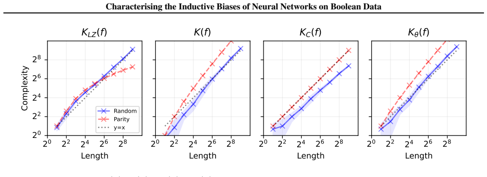
Consider the function f = "1001" × 2n−2. This function is 2-sparse, represented by the DNF (¬x1 ∧ x2) (1 clause, 2 literals). As n increases, its DNF complexity remains fixed at 2. It’s Lempel-Ziv complexity KLZ(f ) = C + log2 n (constant term C for encoding the repeating string and the log n term from the repetitions)

work page
[2]

01001". . . ) KLZ(

However, if we generate a functionf by repeating the string "01001" (truncating at the end) is not ak-sparse function. As a result, its K(f ) will not be constant. See Figure 6 for empirical data showing the discrepancy between these measures. Empirical work in (Valle-Pérez et al., 2018) shows thatK(f ) and KLZ(f ) are correlated. However, they have very ...

work page 2018
[3]

Note that we do not study k-sparse functions in the main text

k-sparse: Generate a random binary string s ∈ {0, 1}2k , then tile it 2n−k times to form the full function string of length 2n. Note that we do not study k-sparse functions in the main text. These are functions generated by repeated patterns of length 2k. In our experiments, we fix n = 7. The parameter grids are: • k-parity: k ∈ {1, 2, . . . ,7}. • t-entr...

work page
[7]

0110" =

Suppose that we train on the first four bits ( m = 4). The minimum norm solution for this is 2-parity (parity on the first two bits). Then, f is just the first 4 bits repeated, 4 x "0110" = "0110011001100110". On the remaining 12 bits, our accuracy is 33%

work page
[8]

01101001

Now we train on the first 8 bits. The minimum norm solution is now 3-parity, 2 x "01101001" = "0110100101101001", which has 0% test accuracy. This argument can be straightforwardly generalised to larger n. Choosing training examples in this way, when trying to 19 Characterising the Inductive Biases of Neural Networks on Boolean Data learn parity generalis...

work page 2019
[9]

, n} of size k, and define: f (x) = L i∈S xi

k-parity: Choose a random subset S ⊆ {1, . . . , n} of size k, and define: f (x) = L i∈S xi

work page
[10]

t-entropy: Select t input points uniformly at random from the 2n possibilities and assign f (x) = 1 on those points (all others map to 0), yielding functions of fixed Hamming weight t

work page
[118]

O’Donnell, R

Springer Science & Business Media, 2012. O’Donnell, R. Analysis of boolean functions. Cambridge University Press, 2014. Olah, C., Cammarata, N., Schubert, L., Goh, G., Petrov, M., and Carter, S. Zoom in: An introduction to circuits. Distill, 5(3):e00024–001, 2020. Olsson, C., Elhage, N., Nanda, N., Joseph, N., DasSarma, N., Henighan, T., Mann, B., Askell,...

arXiv 2012

Show all 12 references

[694]

URL https://proceedings

PMLR, 2020. URL https://proceedings. mlr.press/v119/basri20a.html. ISSN: 2640- 3498. Belkin, M. Fit without fear: remarkable mathematical phe- nomena of deep learning through the prism of interpola- tion, 2021. URL https://arxiv.org/abs/2105. 14368. Bhattamishra, S., Patel, A....

2020 arXiv
[1952]

simplicity bias

URL https://api.semanticscholar. org/CorpusID:124965557. Rahaman, N., Baratin, A., Arpit, D., Draxler, F., Lin, M., Hamprecht, F., Bengio, Y ., and Courville, A. On the spec- tral bias of neural networks. In International Conference on Machine Learning, pp. 5301–5310. PMLR, 20...

2018 arXiv
[2017]

Weight decay

and finds the minimal DNF expression for a given set of inputs that output True. It takes the following arguments: • variables: A list of symbols denoting the literals in the DNF. • minterms: All inputs for which the output of the expression should give True. • dontcares: All ...
[2020]

Chizat, L., Oyallon, E., and Bach, F

URL https://proceedings.mlr.press/ v125/chizat20a.html. Chizat, L., Oyallon, E., and Bach, F. On lazy training in differentiable programming. Advances in neural informa- tion processing systems, 32, 2019. Cohen, O., Malka, O., and Ringel, Z. Learning curves for deep neural net...

2019 arXiv

Pith tools

Reviewed August 7, 2026 · model on record in the stance chip above.

[1] [1]

This function is 2-sparse, represented by the DNF (¬x1 ∧ x2) (1 clause, 2 literals)

Consider the function f = "1001" × 2n−2. This function is 2-sparse, represented by the DNF (¬x1 ∧ x2) (1 clause, 2 literals). As n increases, its DNF complexity remains fixed at 2. It’s Lempel-Ziv complexity KLZ(f ) = C + log2 n (constant term C for encoding the repeating string and the log n term from the repetitions)

work page

[2] [2]

01001". . . ) KLZ(

However, if we generate a functionf by repeating the string "01001" (truncating at the end) is not ak-sparse function. As a result, its K(f ) will not be constant. See Figure 6 for empirical data showing the discrepancy between these measures. Empirical work in (Valle-Pérez et al., 2018) shows thatK(f ) and KLZ(f ) are correlated. However, they have very ...

work page 2018

[3] [3]

Note that we do not study k-sparse functions in the main text

k-sparse: Generate a random binary string s ∈ {0, 1}2k , then tile it 2n−k times to form the full function string of length 2n. Note that we do not study k-sparse functions in the main text. These are functions generated by repeated patterns of length 2k. In our experiments, we fix n = 7. The parameter grids are: • k-parity: k ∈ {1, 2, . . . ,7}. • t-entr...

work page

[4] [7]

0110" =

Suppose that we train on the first four bits ( m = 4). The minimum norm solution for this is 2-parity (parity on the first two bits). Then, f is just the first 4 bits repeated, 4 x "0110" = "0110011001100110". On the remaining 12 bits, our accuracy is 33%

work page

[5] [8]

01101001

Now we train on the first 8 bits. The minimum norm solution is now 3-parity, 2 x "01101001" = "0110100101101001", which has 0% test accuracy. This argument can be straightforwardly generalised to larger n. Choosing training examples in this way, when trying to 19 Characterising the Inductive Biases of Neural Networks on Boolean Data learn parity generalis...

work page 2019

[6] [9]

, n} of size k, and define: f (x) = L i∈S xi

k-parity: Choose a random subset S ⊆ {1, . . . , n} of size k, and define: f (x) = L i∈S xi

work page

[7] [10]

t-entropy: Select t input points uniformly at random from the 2n possibilities and assign f (x) = 1 on those points (all others map to 0), yielding functions of fixed Hamming weight t

work page

[8] [118]

O’Donnell, R

Springer Science & Business Media, 2012. O’Donnell, R. Analysis of boolean functions. Cambridge University Press, 2014. Olah, C., Cammarata, N., Schubert, L., Goh, G., Petrov, M., and Carter, S. Zoom in: An introduction to circuits. Distill, 5(3):e00024–001, 2020. Olsson, C., Elhage, N., Nanda, N., Joseph, N., DasSarma, N., Henighan, T., Mann, B., Askell,...

arXiv 2012