REVIEW 4 major objections 4 minor 86 references
Autoregressive regularized score-based diffusion models for multi-scenarios fluid flow prediction
T0 review · 4 major / 4 minor · reviewed 2026-08-07 · deepseek-v4-flash
Pith's one-line read A regularized score-based diffusion model predicts turbulent flows across varied scenarios.
desk verdict Useful SDE comparison and a genuinely new regularization loss, but the central regularization claim is not identifiable because the ablation retunes noise schedules separately. read the letter →
The pith
A machine-rendered reading of the paper's core claim, the machinery that carries it, and where it could break.
The reading
What carries the argument
The load-bearing ingredients are the autoregressive conditional score-matching objective, the choice among three SDE formulations (variance-preserving, sub-variance-preserving, and variance-exploding), and a regularization term added to the training loss. The regularization decomposes the velocity field into a local mean and fluctuations using two consecutive frames, forms the space-time cross-correlation matrix of the fluctuations, and penalizes the Frobenius-norm difference between predicted and ground-truth correlations, thereby enforcing temporal consistency of turbulent energy statistics at negligible extra cost. The VP SDE, whose diffusion coefficient preserves the total variance of the data distribution, carries the argument by providing a stable noise schedule, and the same U-Net with channel-wise concatenation of the past state is reused for all datasets.
What would settle it
Compute the two-time lag-one autocorrelation of velocity fluctuations, or the FTLE-based Lyapunov time, on any of the three datasets and compare it with the one-step decorrelation assumption; if the lag-one correlation is not near zero, train the regularized and unregularized VP models on that data and check whether the temporal-consistency benefit disappears.
Extended reading notes
Core claim
The central claim is that the regularized variance-preserving SDE (VP SDE) is the most consistently robust and versatile formulation among the score-based diffusion models evaluated, achieving accurate results across multiple scenarios while preserving key physical and statistical properties. The claim is supported by experiments on a two-dimensional compressible transonic cylinder flow, a two-dimensional turbulent radiative layer, and a three-dimensional magnetohydrodynamic flow, where the regularized VP model yields the best or most balanced scores on MSE, Pearson correlation, Kullback-Leibler divergence between field histograms, and log-scale energy-spectrum error. In the harder cases no single formulation dominates every metric, but regularization consistently improves training stability, reduces prediction variance, and improves high-frequency reconstruction. The paper also shows that a Perona-Malik anisotropic diffusion filter applied after generation removes the high-frequency noise that regularization can introduce while preserving coherent vortex structures.
Load-bearing premise
The load-bearing premise is that velocity fluctuations decorrelate within one simulation time step, so the local mean over two consecutive frames gives a valid Reynolds decomposition; if this fails, the regularization weight becomes correlated with the prediction error and the claimed time-consistency benefit collapses.
Editorial extensions
If this is right
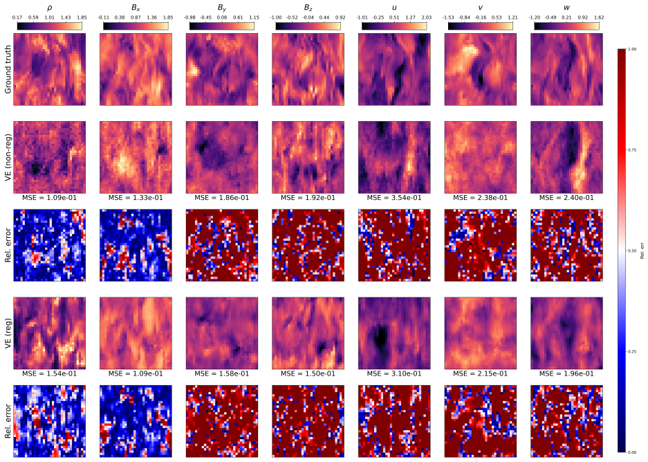
- On the transonic cylinder case, the regularized VP SDE outperforms all other SDE variants on MSE, Pearson correlation, histogram divergence, and log-scale energy-spectrum error, and keeps coherent shock and vortex structures at the final prediction time.
- Regularization stabilizes training and improves low-frequency spectral reconstruction across SDE types, while reducing the spread of predictions across sampled trajectories.
- The VE SDE is the most sensitive to hyperparameter selection and noise, and regularization only partially compensates for its deficiencies at high frequencies.
- Perona-Malik anisotropic filtering after generation removes high-frequency artifacts while preserving Q-criterion structures and vorticity fields, indicating that post-processing can recover physical realism from regularized outputs.
- The same architecture and conditioning mechanism, trained on two-dimensional data, transfers to three-dimensional MHD prediction with minimal modifications, demonstrating plug-and-play applicability.
Reading between the lines
- If the one-step decorrelation assumption holds only because the datasets are sampled at coarse time steps, the regularization may fail on finely sampled simulations where consecutive frames are strongly correlated; this is testable by resampling the same flows at smaller time steps.
- The same correlation-matching penalty could be applied to other generative surrogates, such as flow matching or stochastic interpolants, and to statistical observables beyond velocity, including pressure and magnetic-field correlations.
- The comparisons invite the conclusion that noise-schedule engineering may matter at least as much as architectural sophistication for generative PDE surrogates, a claim the paper does not make explicitly.
- A practical extension is to use the estimated Lyapunov time as a dataset-level criterion for deciding when this regularization is appropriate, since the paper only checks three cases and computes the FTLE on a two-dimensional slice for the three-dimensional case.
Editorial analysis
A structured set of objections, weighed in public.
Referee Report
Summary. The paper proposes an autoregressive conditional score-based diffusion model for multi-scenario fluid flow prediction. The architecture is a U-Net denoiser with channel-wise concatenation of the previous physical frame as conditioning, trained with denoising score matching. The authors compare VP, sub-VP, and VE SDE formulations, introduce a regularization term (Eq. 21) that penalizes a velocity-fluctuation cross-correlation objective, and add a Perona-Malik filter as post-processing. Experiments are carried out on a transonic cylinder, a turbulent radiative layer (TurbRad), and 3D magnetohydrodynamics (MHD) datasets, with MSE, PCC, DKL, log-MSE, energy spectra, and visual diagnostics. The central claim is that the regularized VP SDE is the most consistently robust and versatile formulation and that regularization is crucial for stability and accuracy.
Significance. If the claims hold, the paper would provide a useful contribution: a lightweight, plug-and-play conditioning scheme; a systematic comparison of SDE formulations on public CFD benchmarks; and an explicit energy-weighted regularization with a post-processing filter. Strengths include the use of public datasets, the reproducible hyperparameter table (Table 2), the multi-metric evaluation including log-MSE spectra, and the honest discussion of trade-offs in Sect. 4.5.2. The principal empirical claim, however, is not identifiable from the reported experiments because the regularization comparison is confounded with SDE schedule retuning, and the cross-scenario superiority claim is stronger than the tables support. The contribution is promising but requires controlled experiments and more measured claims before it can be accepted.
major comments (4)
- [Table 2 and Sect. 4.2, Eq. (21)] The claimed benefit of regularization is not identifiable from the reported experiments because the regularized and unregularized models use different SDE noise schedules. For example, for the transonic cylinder VP SDE, beta_min/beta_max are 0.01/5 without regularization versus 0.39/5.6 with regularization; for the MHD VE SDE, sigma_min/sigma_max are 0.1/6 without versus 0.01/4 with. The paper itself notes in Sect. 4.2 that VE is especially sensitive to hyperparameter selection, so any performance difference between a regularized and unregularized pair could be caused by the schedule change rather than by the added loss term in Eq. (21). To support the statement that regularization proves crucial, the authors should provide controlled ablations that fix the schedule (or vary it systematically in both conditions) and report paired results across multiple seeds.
- [Sect. 4.3-4.4, Tables 4-5, Conclusion] The conclusion that the regularized VP SDE emerges as the most consistently robust and versatile formulation is not supported by the aggregated tables. In TurbRad (Table 4), regularized VP has higher MSE than unregularized VP for tc0 and tc2 and higher DKL for tc0 and tc2; in MHD (Table 5), regularized VE has dramatically worse log-MSE than unregularized VE (3.17/4.05 versus 0.40/0.50 for tc1/tc2). The paper acknowledges in Sect. 4.3 that no single formulation dominates across all metrics, yet the abstract and conclusion make a global superiority claim. Please either quantify a rank-based summary across scenarios with uncertainty intervals, or restrict the claim to the cases where the evidence actually holds.
- [Sect. 3.2.3 and Appendix B] The Reynolds decomposition used by the regularizer assumes that velocity fluctuations decorrelate within one simulation time step. The supporting FTLE evidence is heuristic: Appendix B.3 computes FTLE on a 2D slice for the 3D MHD case, uses a heuristically chosen integration time, and reports global Lyapunov times around 0.45-0.51, which are not far below the timestep and come without uncertainty estimates. If the decorrelation assumption fails, the weighting u'(r',tau-1) in Eq. (21) becomes correlated with the prediction error, and the claimed time-consistency benefit collapses. Please provide a direct estimate of the velocity autocorrelation timescale from the data, or present the regularizer as an ad hoc weighting rather than a physics-derived constraint.
- [Eq. (21) and Sect. 4.2] The regularizer is trained with teacher forcing: the term D(u, hat u) uses the ground-truth previous frame, hat u(r,tau-1) identified with u(r,tau-1), but at inference the conditioning input is the model's own previous prediction. The paper does not discuss this distribution mismatch, although the claimed stabilization of autoregressive rollouts depends on the regularizer's effect transferring to free-running conditions. Please add an analysis of this gap, for example scheduled sampling or a comparison of error accumulation with and without regularization, or explicitly state this as a limitation.
minor comments (4)
- [Sect. 3.2.3] The text refers to a 'Fischer-like divergence'; this should be 'Fisher-like divergence'.
- [Eq. (20)] The notation in Eq. (20) mixes the discrete diffusion index i with the continuous-time convention used elsewhere; please align the notation, using for example x_tau_t, and clarify the relationship between temb and t.
- [Eq. (22) and surrounding text] The statement that the inertial-subrange scaling kappa^{-5/3} holds 'either in 2D or in 3D' is an oversimplification of 2D turbulence phenomenology; please qualify this claim.
- [Sect. 4.1 and Tables 3-5] The hyperparameter search uses random search and early stopping, but no number of seeds or repeated runs is reported, so the tables give point estimates without uncertainty; please state how many seeds were used and report the corresponding variability.
Circularity Check
No significant circularity: the regularized score-based model is trained with an extra data-dependent loss term, and the reported evaluations are external to the training objective.
full rationale
The paper's derivation chain is empirical rather than definitional. The baseline objective L_AM in Eq. (15) is the standard conditional denoising score-matching loss, and the regularization in Eq. (21) adds an explicit weighted squared-error term on the velocity fluctuations (Sect. 3.2.3). The regularizer uses the ground-truth previous frame during training (u-hat(r, tau-1) = u(r, tau-1)), which is teacher forcing, not a circular construction: the reported metrics (MSE, PCC, DKL, log-MSE, energy spectra) are computed against held-out test cases and are not equal by construction to the regularizer or to the training objective. The claim that regularized VP SDE is most robust is a comparative empirical conclusion, and the paper's own results show mixed evidence (e.g., TurbRad and MHD do not show uniform dominance, and Sect. 4.5.2 shows regularized raw outputs can be noisier). This is an experimental-identifiability concern, especially because Table 2 retunes SDE hyperparameters separately for regularized and unregularized models, but it is not circularity: no fitted parameter is renamed as a prediction, and no result is forced by a self-citation chain. The paper contains no load-bearing self-citations; references to prior work such as Kohl et al. [36], Shysheya et al. [35], and Song et al. [54] are external foundations, and the cited 'provably efficient autoregressive framework' is not used to forbid alternatives or to justify the regularizer. The FTLE-based decorrelation assumption (Appendix B) is a support weakness, not a circular step. Overall, the derivation is self-contained and the central claims rest on independent experiments, so the circularity score is 0.
Assumptions & free parameters
free parameters (5)
- Regularization weight λw =
not reported
- SDE noise schedule bounds =
Table 2 values (e.g., VP: βmin=0.01, βmax=5 for transonic cylinder)
- Perona-Malik filter parameters =
γ=0.05, η=0.03, ε=1e-8, N unspecified
- FTLE integration time Δτ =
not reported, heuristically adjusted
- Training epochs =
600 (cylinder), 700 (TurbRad), 70 (MHD)
assumptions (4)
- standard math Score-based diffusion theory, including Anderson's time reversal and denoising score matching equivalence, holds.
- domain assumption The velocity field can be decomposed into a local mean over two frames and a zero-mean fluctuating component, with fluctuations decorrelating within one time step.
- domain assumption Using only the immediately previous state (m=1) is sufficient for autoregressive conditioning.
- domain assumption The datasets are large enough to treat sampled states as approximately i.i.d.
Cite this review
Pith. "Pith review of Autoregressive regularized score-based diffusion models for multi-scenarios fluid flow prediction." pith.science (2026). https://pith.science/paper/CKDXXUI5
@misc{pith2026250524145,
  author       = {Pith},
  title        = {Pith review of: Autoregressive regularized score-based diffusion models for multi-scenarios fluid flow prediction},
  year         = {2026},
  howpublished = {\url{https://pith.science/paper/CKDXXUI5}},
  note         = {Machine review of arXiv:2505.24145}
}
read the original abstract
Building on recent advances in scientific machine learning and generative modeling for computational fluid dynamics, we propose a conditional score-based diffusion model designed for multi-scenarios fluid flow prediction. Our model integrates an energy constraint rooted in the statistical properties of turbulent flows, improving prediction quality with minimal training, while enabling efficient sampling at low cost. The method features a simple and general architecture that requires no problem-specific design, supports plug-and-play enhancements, and enables fast and flexible solution generation. It also demonstrates an efficient conditioning mechanism that simplifies training across different scenarios without demanding a redesign of existing models. We further explore various stochastic differential equation formulations to demonstrate how thoughtful design choices enhance performance. We validate the proposed methodology through extensive experiments on complex fluid dynamics datasets encompassing a variety of flow regimes and configurations. Results demonstrate that our model consistently achieves stable, robust, and physically faithful predictions, even under challenging turbulent conditions. With properly tuned parameters, it achieves accurate results across multiple scenarios while preserving key physical and statistical properties. We present a comprehensive analysis of stochastic differential equation impact and discuss our approach across diverse fluid mechanics tasks.
Figures


Figures from the paper (7 more)




Reference graph
Works this paper leans on
-
[1]
Numerical Computation of Internal and External Flows
Charles Hirsch. Numerical Computation of Internal and External Flows . Butterworth-Heinemann, Oxford, second edition, 2007. doi: 10.1016/B978-0-7506-6594-0.X5037-1
-
[2]
Stephen B. Pope. Turbulent Flows. Cambridge University Press, Cambridge, first edition, 2000. doi: 10.1017 /CBO9780511840531
2000
-
[3]
Direct numerical simulation: a tool in turbulence research
Parviz Moin and Krishnan Mahesh. Direct numerical simulation: a tool in turbulence research. Annual Review of Fluid Mechanics, 30(1): 539–578, 1998. doi: 10.1146 /annurev.fluid.30.1.539
1998
-
[4]
Turbulence modeling and simulation advances in CFD during the past 50 years
Roland Schiestel and Bruno Chaouat. Turbulence modeling and simulation advances in CFD during the past 50 years. Comptes Rendus. M´ ecanique, 350(S1):23–51, 2022. doi: 10.5802 /crmeca.114
2022
-
[5]
Brunton, Bernd R
Steven L. Brunton, Bernd R. Noack, and Petros Koumoutsakos. Machine learning for fluid mechanics. Annual Review of Fluid Mechanics, 52:477–508, 2020. doi: 10.1146 /annurev-fluid-010719-060214
2020
-
[6]
Data reconstruction for complex flows using AI: Recent progress, obstacles, and perspectives
Michele Buzzicotti. Data reconstruction for complex flows using AI: Recent progress, obstacles, and perspectives. Europhysics Letters, 142 (2):23001, 2023. doi: 10.1209 /0295-5075/acc88c
2023
-
[7]
Turbulence modeling in the age of data
Karthik Duraisamy, Gianluca Iaccarino, and Heng Xiao. Turbulence modeling in the age of data. Annual Review of Fluid Mechanics , 51: 357–377, 2019. doi: 10.1146 /annurev-fluid-010518-040547
2019
-
[8]
Mario Lino, Stathi Fotiadis, Anil A. Bharath, and Chris D. Cantwell. Current and emerging deep-learning methods for the simulation of fluid dynamics. Proceedings of the Royal Society A: Mathematical, Physical and Engineering Sciences , 479(2275):20230058, 2023. doi: 10.1098/rspa.2023.0058
arXiv 2023
Show all 86 references
-
[9]
Ricardo Vinuesa and Steven L. Brunton. Enhancing computational fluid dynamics with machine learning. Nature Computational Science, 2 (6):358–366, 2022. doi: 10.1038 /s43588-022-00264-7
2022
-
[10]
Karniadakis
Maziar Raissi, Paris Perdikaris, and George E. Karniadakis. Physics-informed neural networks: A deep learning framework for solving forward and inverse problems involving nonlinear partial differential equations. Journal of Computational Physics, 378:686–707, 2019
2019
-
[11]
Likas, and Dimitrios I
Isaac Elias Lagaris, Aristidis C. Likas, and Dimitrios I. Fotiadis. Artificial neural networks for solving ordinary and partial di fferential equations. IEEE Transactions on Neural Networks, 9(5):987–1000, 1998. doi: 10.1109 /72.712178
1998
-
[12]
Likas, and Dimitrios G
Isaac Elias Lagaris, Aristidis C. Likas, and Dimitrios G. Papageorgiou. Neural-network methods for boundary value problems with irregular boundaries. IEEE Transactions on Neural Networks, 11(5):1041–1049, 2000. doi: 10.1109 /72.870037
-
[13]
The graph neural network model
Franco Scarselli, Marco Gori, Ah Chung Tsoi, Markus Hagenbuchner, and Gabriele Monfardini. The graph neural network model. IEEE Transactions on Neural Networks, 20(1):61–80, 2009. doi: 10.1109 /TNN.2008.2005605
2009
-
[14]
Fourier neural operator for parametric partial differential equations
Zongyi Li, Nikola Kovachki, Kamyar Azizzadenesheli, Burigede Liu, Kaushik Bhattacharya, Andrew Stuart, and Anima Anandkumar. Fourier neural operator for parametric partial differential equations. arXiv:2010.08895, 2021
2010 arXiv
-
[15]
Prediction of turbulent channel flow using Fourier neural operator-based machine-learning strategy
Yunpeng Wang, Zhijie Li, Zelong Yuan, Wenhui Peng, Tianyuan Liu, and Jianchun Wang. Prediction of turbulent channel flow using Fourier neural operator-based machine-learning strategy. Physical Review Fluids, 9(8):084604, 2024
2024
-
[16]
Universal approximation to nonlinear operators by neural networks with arbitrary activation functions and its application to dynamical systems
Tianping Chen and Hong Chen. Universal approximation to nonlinear operators by neural networks with arbitrary activation functions and its application to dynamical systems. IEEE Transactions on Neural Networks, 6(4):911–917, 1995. doi: 10.1109 /72.392253
1995
-
[17]
Karniadakis
Lu Lu, Pengzha10.1007 /BF02128236n Jin, Guofei Pang, Zhongqiang Zhang, and George E. Karniadakis. Learning nonlinear operators via DeepONet based on the universal approximation theorem of operators. Nature Machine Intelligence, 3(3):218–229, 2021. doi: 10.1038 / s42256-021-00302-5
-
[18]
Poseidon: Efficient foundation models for PDEs
Maximilian Herde, Bogdan Raoni ´c, Tobias Rohner, Roger K ¨appeli, Roberto Molinaro, Emmanuel de B ´ezenac, and Siddhartha Mishra. Poseidon: Efficient foundation models for PDEs. arXiv:2405.19101, 2024
2024 arXiv
-
[19]
PDE-Refiner: Achieving accurate long rollouts with neural PDE solvers
Phillip Lippe, Bas Veeling, Paris Perdikaris, Richard Turner, and Johannes Brandstetter. PDE-Refiner: Achieving accurate long rollouts with neural PDE solvers. Advances in Neural Information Processing Systems, 36:67398–67433, 2023
2023
-
[20]
Hou, and Max Tegmark
Ziming Liu, Yixuan Wang, Sachin Vaidya, Fabian Ruehle, James Halverson, Marin Solja ˇci´c, Thomas Y . Hou, and Max Tegmark. KAN: Kolmogorov-Arnold Networks. arXiv:2404.19756, 2025
2025 arXiv
-
[21]
Karniadakis
Juan Diego Toscano, Theo K ¨aufer, Zhibo Wang, Martin Maxey, Christian Cierpka, and George E. Karniadakis. Inferring turbulent velocity and temperature fields and their statistics from Lagrangian velocity measurements using physics-informed Kolmogorov-Arnold networks. arXiv:24...
2024 arXiv
-
[22]
Goodfellow, Jean Pouget-Abadie, Mehdi Mirza, Bing Xu, David Warde-Farley, Sherjil Ozair, Aaron Courville, and Yoshua Bengio
Ian J. Goodfellow, Jean Pouget-Abadie, Mehdi Mirza, Bing Xu, David Warde-Farley, Sherjil Ozair, Aaron Courville, and Yoshua Bengio. Generative adversarial nets. arXiv:1406.2661, 2014
2014 arXiv
-
[23]
Generative modeling of turbulence
Claudia Drygala, Benjamin Winhart, Frencesca di Mare, and Hanno Gottschalk. Generative modeling of turbulence. Physics of Fluids, 34 (3):035114, 2022. doi: 10.1063 /5.0082562
2022
-
[24]
Kingma and Max Welling
Diederik P. Kingma and Max Welling. Auto-encoding variational Bayes. arXiv:1312.6114, 2013
2013 arXiv
-
[25]
Deep unsupervised learning using nonequilibrium thermo- dynamics
Jascha Sohl-Dickstein, Eric Weiss, Niru Maheswaranathan, and Surya Ganguli. Deep unsupervised learning using nonequilibrium thermo- dynamics. In International Conference on Machine Learning, pages 2256–2265. PMLR, 2015
2015
-
[26]
Denoising di ffusion probabilistic models
Jonathan Ho, Ajay Jain, and Pieter Abbeel. Denoising di ffusion probabilistic models. Advances in Neural Information Processing Systems, 33:6840–6851, 2020
2020
-
[27]
Comparison of generative learning methods for turbulence modeling
Claudia Drygala, Edmund Ross, Francesca di Mare, and Hanno Gottschalk. Comparison of generative learning methods for turbulence modeling. arXiv:2411.16417, 2024
2024
-
[28]
Neural di fferentiable modeling with diffusion-based super-resolution for two-dimensional spatiotemporal turbulence
Xiantao Fan, Deepak Akhare, and Jian-Xun Wang. Neural di fferentiable modeling with diffusion-based super-resolution for two-dimensional spatiotemporal turbulence. Computer Methods in Applied Mechanics and Engineering, 433:117478, 2025
2025
-
[29]
From zero to turbulence: Generative modeling for 3D flow simulation
Marten Lienen, David L ¨udke, Jan Hansen-Palmus, and Stephan G ¨unnemann. From zero to turbulence: Generative modeling for 3D flow simulation. arXiv:2306.01776, 2023
2023 arXiv
-
[30]
Prince, and Marcus A
Ivan Kobyzev, Simon J.D. Prince, and Marcus A. Brubaker. Normalizing flows: An introduction and review of current methods. IEEE Transactions on Pattern Analysis and Machine Intelligence, 43(11):3964–3979, 2020
2020
-
[31]
Chen, Heli Ben-Hamu, Maximilian Nickel, and Matt Le
Yaron Lipman, Ricky T.Q. Chen, Heli Ben-Hamu, Maximilian Nickel, and Matt Le. Flow matching for generative modeling. arXiv:2210.02747, 2022. 32
2022 arXiv
-
[32]
Chen, Yulia Rubanova, Jesse Bettencourt, and David Duvenaud
Ricky T.Q. Chen, Yulia Rubanova, Jesse Bettencourt, and David Duvenaud. Neural ordinary differential equations. arXiv:1806.07366, 2018
2018 arXiv
-
[33]
Di ffusion schr ¨odinger bridge with applications to score-based generative modeling
Valentin de Bortoli, James Thornton, Jeremy Heng, and Arnaud Doucet. Di ffusion schr ¨odinger bridge with applications to score-based generative modeling. Advances in Neural Information Processing Systems, 34:17695–17709, 2021
2021
-
[34]
Stochastic interpolants: A unifying framework for flows and di ffusions
Michael S Albergo, Nicholas M Bo ffi, and Eric Vanden-Eijnden. Stochastic interpolants: A unifying framework for flows and di ffusions. arXiv:2303.08797, 2023
2023 arXiv
-
[35]
On conditional diffusion models for PDE simulations.Advances in Neural Information Processing Systems, 37:23246–23300, 2024
Aliaksandra Shysheya, Cristiana Diaconu, Federico Bergamin, Paris Perdikaris, Jos ´e Miguel Hern´andez-Lobato, Richard Turner, and Emile Mathieu. On conditional diffusion models for PDE simulations.Advances in Neural Information Processing Systems, 37:23246–23300, 2024
2024
-
[36]
Benchmarking autoregressive conditional di ffusion models for turbulent flow simulation
Georg Kohl, Li-Wei Chen, and Nils Thuerey. Benchmarking autoregressive conditional di ffusion models for turbulent flow simulation. arXiv:2309.01745, 2023
2023 arXiv
-
[37]
Di ffusionPDE: Generative PDE-solving under partial observation
Jiahe Huang, Guandao Yang, Zichen Wang, and Jeong Joon Park. Di ffusionPDE: Generative PDE-solving under partial observation. arXiv:2406.17763, 2024
2024 arXiv
-
[38]
CoNFiLD: Conditional neural field latent di ffusion model generating spatiotemporal turbulence
Pan Du, Meet Hemant Parikh, Xiantao Fan, Xin-Yang Liu, and Jian-Xun Wang. CoNFiLD: Conditional neural field latent di ffusion model generating spatiotemporal turbulence. arXiv:2403.05940, 2024
2024 arXiv
-
[39]
Andersson, Andrew El-Kadi, Dominic Masters, Timo Ewalds, Jacklynn Stott, Shakir Mohamed, Peter Battaglia, Remi Lam, and Matthew Willson
Ilan Price, Alvaro Sanchez-Gonzalez, Ferran Alet, Tom R. Andersson, Andrew El-Kadi, Dominic Masters, Timo Ewalds, Jacklynn Stott, Shakir Mohamed, Peter Battaglia, Remi Lam, and Matthew Willson. Probabilistic weather forecasting with machine learning. Nature, 637: 84–90, 2025. ...
2025
-
[40]
Janik, and Yaron Oz
Tim Whittaker, Romuald A. Janik, and Yaron Oz. Turbulence scaling from deep learning di ffusion generative models. Journal of Computa- tional Physics, 514:113239, 2024. doi: 10.1016 /j.jcp.2024.113239
2024
-
[41]
DYffusion: A dynamics-informed diffusion model for spatiotemporal forecasting
Salva R ¨uhling Cachay, Bo Zhao, Hailey Joren, and Rose Yu. DYffusion: A dynamics-informed diffusion model for spatiotemporal forecasting. Advances in Neural Information Processing Systems, 36:45259–45287, 2023
2023
-
[42]
Pi-fusion: Physics-informed di ffusion model for learning fluid dynamics
Jing Qiu, Jiancheng Huang, Xiangdong Zhang, Zeng Lin, Minglei Pan, Zengding Liu, and Fen Miao. Pi-fusion: Physics-informed di ffusion model for learning fluid dynamics. arXiv:2406.03711, 2024
2024 arXiv
-
[43]
Physics-informed di ffusion models
Jan-Hendrik Bastek, WaiChing Sun, and Dennis M Kochmann. Physics-informed di ffusion models. arXiv:2403.14404, 2024
2024 arXiv
-
[44]
A physics-informed di ffusion model for high-fidelity flow field reconstruction
Dule Shu, Zijie Li, and Amir Barati Farimani. A physics-informed di ffusion model for high-fidelity flow field reconstruction. Journal of Computational Physics, 478:111972, 2023
2023
-
[45]
A denoising di ffusion model for fluid field prediction
Gefan Yang and Stefan Sommer. A denoising di ffusion model for fluid field prediction. arXiv:2301.11661, 2023
2023 arXiv
-
[46]
Conditional score-based diffusion models for solving inverse problems in mechanics
Agnimitra Dasgupta, Harisankar Ramaswamy, Javier Murgoitio Esandi, Ken Foo, Runze Li, Qifa Zhou, Brendan Kennedy, and Assad Oberai. Conditional score-based diffusion models for solving inverse problems in mechanics. arXiv:2406.13154, 2024
2024 arXiv
-
[47]
Generative learning of the solution of parametric partial di fferential equations using guided diffusion models and virtual observations
Han Gao, Sebastian Kaltenbach, and Petros Koumoutsakos. Generative learning of the solution of parametric partial di fferential equations using guided diffusion models and virtual observations. Computer Methods in Applied Mechanics and Engineering, 435:117654, 2025
2025
-
[48]
CoCoGen: Physically consistent and conditioned score-based generative models for forward and inverse problems
Christian Jacobsen, Yilin Zhuang, and Karthik Duraisamy. CoCoGen: Physically consistent and conditioned score-based generative models for forward and inverse problems. SIAM Journal on Scientific Computing, 47(2):C399–C425, 2025
2025
-
[49]
Adding conditional control to text-to-image di ffusion models
Lvmin Zhang, Anyi Rao, and Maneesh Agrawala. Adding conditional control to text-to-image di ffusion models. In Proceedings of the IEEE/CVF international conference on computer vision, pages 3836–3847, 2023
2023
-
[50]
Physics-informed score-based diffusion model for limited-angle reconstruction of cardiac computed tomography
Shuo Han, Yongshun Xu, Dayang Wang, Bahareh Morovati, Li Zhou, Jonathan S Maltz, Ge Wang, and Hengyong Yu. Physics-informed score-based diffusion model for limited-angle reconstruction of cardiac computed tomography. arXiv:2405.14770, 2024
2024 arXiv
-
[51]
M ¨ucke and Benjamin Sanderse
Nikolaj T. M ¨ucke and Benjamin Sanderse. Physics-aware generative models for turbulent fluid flows through energy-consistent stochastic interpolants. arXiv:2504.05852, 2025
2025 arXiv
-
[52]
Fielding, Eve C
Drummond B. Fielding, Eve C. Ostriker, Greg L. Bryan, and Adam S. Jermyn. Multiphase gas and the fractal nature of radiative turbulent mixing layers. The Astrophysical Journal Letters, 894(2):L24, 2020
2020
-
[53]
Appel, Shmuel Bialy, Jungyeon Cho, Andrew J
Blakesley Burkhart, Sabrina M. Appel, Shmuel Bialy, Jungyeon Cho, Andrew J. Christensen, David Collins, Christoph Federrath, Drum- mond B. Fielding, Douglas Finkbeiner, Alex S. Hill, Juan Camilo Ib ´a˜nez Mej´ıa, Mark R. Krumholz, Alexandre Lazarian, Miao Li, Philip Mocz, Mord...
2020
-
[54]
Score-based generative modeling through stochastic differential equations
Yang Song, Jascha Sohl-Dickstein, Diederik P Kingma, Abhishek Kumar, Stefano Ermon, and Ben Poole. Score-based generative modeling through stochastic differential equations. arXiv:2011.13456, 2020
2011 arXiv
-
[55]
Christophe Andrieu, Nando de Freitas, Arnaud Doucet, and Michael I. Jordan. An introduction to MCMC for machine learning. Machine Learning, 50(1):5–43, 2003. doi: 10.1023 /A:1020281327116
2003
-
[56]
Understanding di ffusion models: A unified perspective
Calvin Luo. Understanding di ffusion models: A unified perspective. arXiv:2208.11970, 2022
2022 arXiv
-
[57]
U-Net: Convolutional networks for biomedical image segmentation
Olaf Ronneberger, Philipp Fischer, and Thomas Brox. U-Net: Convolutional networks for biomedical image segmentation. In Medical image computing and computer-assisted intervention–MICCAI 2015: 18th international conference, Munich, Germany, October 5-9, 2015, proceedings, part ...
2015 doi
-
[58]
Estimation of non-normalized statistical models by score matching
Aapo Hyv ¨arinen. Estimation of non-normalized statistical models by score matching. Journal of Machine Learning Research, 6(4):695–709, 2005
2005
-
[59]
Generative modeling by estimating gradients of the data distribution
Yang Song and Stefano Ermon. Generative modeling by estimating gradients of the data distribution. Advances in Neural Information Processing Systems, 32, 2019
2019
-
[60]
Stochastic Differential Equations: an Introduction with Applications
Bernt Øksendal. Stochastic Differential Equations: an Introduction with Applications. Springer Science & Business Media, Berlin, 2013
2013
-
[61]
Applied Stochastic Differential Equations, volume 10
Simo S ¨arkk¨a and Arno Solin. Applied Stochastic Differential Equations, volume 10. Cambridge University Press, Cambridge, 2019
2019
-
[62]
Anderson
Brian D.O. Anderson. Reverse-time di ffusion equation models. Stochastic Processes and their Applications, 12(3):313–326, 1982
1982
-
[63]
Time reversal of diffusion processes under a finite entropy condition
Patrick Cattiaux, Giovanni Conforti, Ivan Gentil, and Christian L´eonard. Time reversal of diffusion processes under a finite entropy condition. Annales de l’Institut Henri Poincar´ e (B) Probabilit´ es et Statistiques, 59(4):1844–1881, 2023. doi: 10.1214 /22-AIHP1320
2023
-
[64]
Haussmann and ´Etienne Pardoux
Ulrich G. Haussmann and ´Etienne Pardoux. Time reversal of di ffusions. The Annals of Probability, pages 1188–1205, 1986. doi: 10.1214 / aop/1176992362
1986
-
[65]
Sliced score matching: A scalable approach to density and score estimation
Yang Song, Sahaj Garg, Jiaxin Shi, and Stefano Ermon. Sliced score matching: A scalable approach to density and score estimation. In Uncertainty in Artificial Intelligence, pages 574–584. PMLR, 2020. 33
2020
-
[66]
Improved techniques for training score-based generative models
Yang Song and Stefano Ermon. Improved techniques for training score-based generative models. Advances in Neural Information Processing Systems, 33:12438–12448, 2020
2020
-
[67]
A connection between score matching and denoising autoencoders
Pascal Vincent. A connection between score matching and denoising autoencoders. Neural Computation, 23(7):1661–1674, 2011
2011
-
[68]
A variational perspective on diffusion-based generative models and score matching
Chin-Wei Huang, Jae Hyun Lim, and Aaron C Courville. A variational perspective on diffusion-based generative models and score matching. Advances in Neural Information Processing Systems, 34:22863–22876, 2021
2021
-
[69]
Variational di ffusion models
Diederik Kingma, Tim Salimans, Ben Poole, and Jonathan Ho. Variational di ffusion models. Advances in Neural Information Processing Systems, 34:21696–21707, 2021
2021
-
[70]
Maximum likelihood training of score-based di ffusion models
Yang Song, Conor Durkan, Iain Murray, and Stefano Ermon. Maximum likelihood training of score-based di ffusion models. Advances in Neural Information Processing Systems, 34:1415–1428, 2021
2021
-
[71]
Elucidating the design space of di ffusion-based generative models
Tero Karras, Miika Aittala, Timo Aila, and Samuli Laine. Elucidating the design space of di ffusion-based generative models. Advances in Neural Information Processing Systems, 35:26565–26577, 2022
2022
-
[72]
Improved techniques for maximum likelihood estimation for di ffusion ODEs
Kaiwen Zheng, Cheng Lu, Jianfei Chen, and Jun Zhu. Improved techniques for maximum likelihood estimation for di ffusion ODEs. In International Conference on Machine Learning, pages 42363–42389. PMLR, 2023
2023
-
[73]
A probabilistic generative model for semi-supervised training of coarse-grained surrogates and enforcing physical constraints through virtual observables
Maximilian Rixner and Phaedon-Stelios Koutsourelakis. A probabilistic generative model for semi-supervised training of coarse-grained surrogates and enforcing physical constraints through virtual observables. Journal of Computational Physics, 434:110218, 2021
2021
-
[74]
A score-based generative solver for PDE-constrained inverse problems with complex priors
Yankun Hong, Harshit Bansal, and Karen Veroy. A score-based generative solver for PDE-constrained inverse problems with complex priors. arXiv:2408.16626, 2024
2024 arXiv
-
[75]
Classifier-free di ffusion guidance
Jonathan Ho and Tim Salimans. Classifier-free di ffusion guidance. arXiv:2207.12598, 2022
2022 arXiv
-
[76]
Unveil conditional di ffusion models with classifier-free guidance: A sharp statistical theory
Hengyu Fu, Zhuoran Yang, Mengdi Wang, and Minshuo Chen. Unveil conditional di ffusion models with classifier-free guidance: A sharp statistical theory. arXiv:2403.11968, 2024
2024 arXiv
-
[77]
Conditional image generation with score-based diffusion models
Georgios Batzolis, Jan Stanczuk, Carola-Bibiane Sch ¨onlieb, and Christian Etmann. Conditional image generation with score-based diffusion models. arXiv:2111.13606, 2021
2021 arXiv
-
[78]
Economon, Francisco Palacios, Sean R
Thomas D. Economon, Francisco Palacios, Sean R. Copeland, Trent W. Lukaczyk, and Juan J. Alonso. SU2: An open-source suite for multiphysics simulation and design. AIAA Journal, 54(3):828–846, 2016
2016
-
[79]
Goldberg, Keiya Hirashima, Yan-Fei Jiang, Rich R
Ruben Ohana, Michael McCabe, Lucas Meyer, Rudy Morel, Fruzsina Agocs, Miguel Beneitez, Marsha Berger, Blakesly Burkhart, Stuart Dalziel, Drummond Fielding, Daniel Fortunato, Jared A. Goldberg, Keiya Hirashima, Yan-Fei Jiang, Rich R. Kerswell, Suryanarayana Maddu, Jonah Miller,...
2024
-
[80]
Gomez, Lukasz Kaiser, and Illia Polosukhin
Ashish Vaswani, Noam Shazeer, Niki Parmar, Jakob Uszkoreit, Llion Jones, Aidan N. Gomez, Lukasz Kaiser, and Illia Polosukhin. Attention is all you need. arXiv:1706.03762, 2023
2023 arXiv
-
[81]
Image-to-image translation with conditional adversarial networks
Phillip Isola, Jun-Yan Zhu, Tinghui Zhou, and Alexei A Efros. Image-to-image translation with conditional adversarial networks. In Pro- ceedings of the IEEE Conference on Computer Vision and Pattern Recognition, pages 1125–1134, 2017
2017
-
[82]
Lyapunov characteristic exponents for smooth dynamical systems and for hamiltonian systems; a method for computing all of them
Giancarlo Benettin, Luigi Galgani, Antonio Giorgilli, and Jean-Marie Strelcyn. Lyapunov characteristic exponents for smooth dynamical systems and for hamiltonian systems; a method for computing all of them. Part 1: Theory. Meccanica, 15:9–20, 1980. doi: 10.1007 / BF02128236
1980
-
[83]
Robinson
James C. Robinson. The Navier-Stokes regularity problem. Philosophical Transactions of the Royal Society A: Mathematical, Physical and Engineering Sciences, 378(2174):20190526, 2020. doi: 10.1098 /rsta.2019.0526
2020
-
[84]
Pearson correlation coe fficient
Jacob Benesty, Jingdong Chen, Yiteng Huang, and Israel Cohen. Pearson correlation coe fficient. In Noise Reduction in Speech Processing, pages 1–4. Springer, Berlin, 2009. doi: 10.1007/978-3-642-00296-0 5
2009 doi
-
[85]
On coherent-vortex identification in turbulence
Yves Dubief and Franck Delcayre. On coherent-vortex identification in turbulence. Journal of Turbulence, 1(11):011, 2000. doi: 10.1088 / 1468-5248/1/1/011
2000
-
[86]
Scale-space and edge detection using anisotropic di ffusion
Pietro Perona and Jitendra Malik. Scale-space and edge detection using anisotropic di ffusion. IEEE Transactions on Pattern Analysis and Machine Intelligence, 12(7):629–639, 1990. doi: 10.1109 /34.56205. 34
1990
Reviewed August 7, 2026 · model on record in the stance chip above.
Discussion (0). Sign in to comment.