REVIEW 4 major objections 5 minor 47 references
Predicting the Past: Estimating Historical Appraisals with OCR and Machine Learning
T0 review · 4 major / 5 minor · reviewed 2026-08-07 · deepseek-v4-flash
Pith's one-line read This paper develops a cost-effective OCR and machine-learning pipeline that digitizes handwritten 1933 property assessment cards at scale, produces the first county-wide dataset of historical appraisals for Hamilton County, Ohio, and…
desk verdict A useful public dataset and a solid OCR pipeline, undercut by an unverified proxy assumption in the regression half and a cross-county test that is partly calibrated to the target county's own labels. read the letter →
The pith
A machine-rendered reading of the paper's core claim, the machinery that carries it, and where it could break.
The reading
What carries the argument
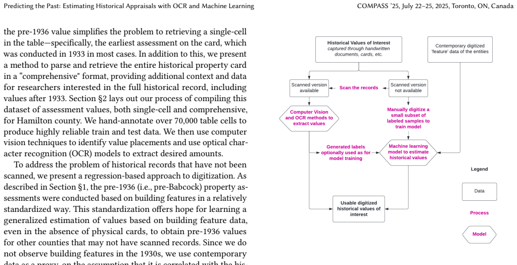
The workhorse is a two-stage tabular extraction pipeline: first align the scanned card to a blank template using ORB feature matching and a RANSAC homography so every table cell has a known position, then read each cropped cell with a fine-tuned TrOCR model; a separate single-cell variant locates the BUILDINGS column header with Tesseract and uses a Hough transform to isolate the first valuation cell. When a card cannot be read, a random-forest regressor trained on contemporary building features (square footages, stories, grade, wall type, rooms, baths, garage capacity, and similar attributes) predicts the 1933 value, and a location-scale shift, Equation 1, adjusts the prediction to another county's value distribution.
What would settle it
Compare the contemporary features used by the model (square footage, room counts, wall type) against the features recorded on the original 1933 cards for a random sample of parcels; if parcels with measurable feature changes show prediction errors systematically above those without changes, the proxy assumption fails.
Extended reading notes
Core claim
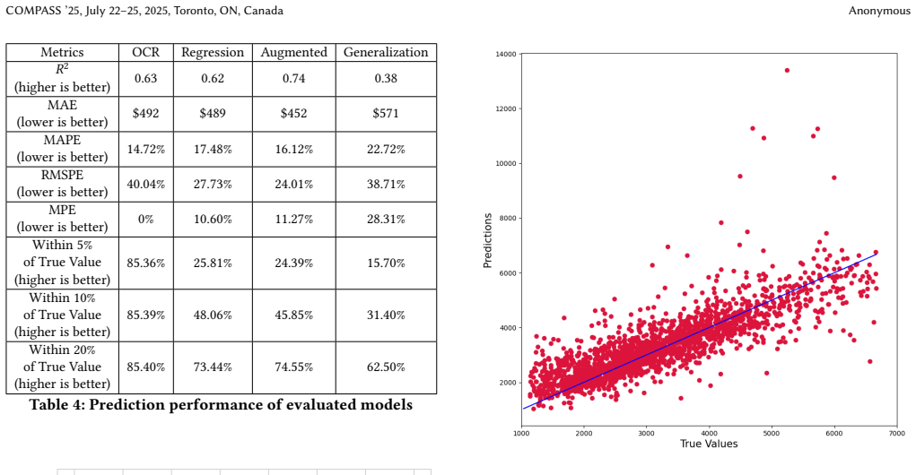
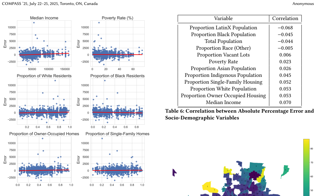
The first county-wide dataset of historical property assessments, constructed from scanned cards, is the paper's central deliverable, together with a regression model that can extrapolate the same quantity to counties without scans. The authors claim that their pipeline, which aligns a scan to a fixed template using ORB feature matching and a RANSAC homography, segments table cells with a Hough transform, and reads digits with a fine-tuned TrOCR transformer, extracts the 1933 building valuation from handwritten cards with 85% of predictions within 5% of the true value and a 5.42% MAPE on the top 90% of confident outputs. The regression model, a random forest trained on contemporary parcel and building data, reaches 17.48% MAPE on held-out Hamilton County properties, improves to 16.12% when OCR labels are added at a confidence threshold, and transfers to Franklin County at 22.72% MAPE after a location-scale correction estimated from 100 labeled parcels. The authors further report near-zero correlation between prediction error and tract-level income, race, and housing variables, and no bias from the roughly 5.6% of parcels whose cards were missing.
Load-bearing premise
Contemporary building records from the 2020s are a dependable stand-in for the size and features a house had in 1933, so a model trained on today's features can estimate a 1933 appraisal.
Editorial extensions
If this is right
- A researcher can now download the released Hamilton County 1933 building appraisals and compare them with redlining maps, sale prices, and demographic data to estimate the policy's immediate financial consequences.
- Counties without scanned cards can obtain rough pre-1936 estimates from contemporary assessor data at 17% to 23% typical error, enabling multi-city studies without archival scanning.
- The fixed-layout alignment-and-segment recipe transfers to other tabular historical records such as tax rolls, censuses, and business directories at an estimated 78% cost saving over manual entry.
- Because the paper finds no meaningful error gradient across census-tract demographics, downstream inequality analyses can use the predicted values without a built-in demographic bias in the errors.
- The released code and dataset allow social scientists to reproduce the digitization and extend the regression to other jurisdictions rather than re-scan archives from scratch.
Reading between the lines
- The paper does not test how many ground-truth labels are needed per new county beyond the 100 used for the location-scale shift; a low-cost robustness check would be fitting the same model with 25, 50, and 200 Franklin labels and seeing whether the 22.72% error stabilizes.
- Because the regression relies on today's features as a proxy for 1933 features, neighborhoods with high rates of renovation, demolition, or postwar construction will likely show larger errors than the reported aggregates suggest, so per-parcel use of the regression estimates should be treated cautiously.
- The pipeline could be run on the same cards after 1933, not just the earliest entry, so the method can quantify how appraisal gaps widened after the 1936 Federal Underwriting Manual rather than only establishing the pre-redlining baseline.
- The heavy-tailed OCR errors (occasional inserted or deleted digits) make point estimates for individual parcels risky; the confidence-threshold filtering the paper applies is essential for any per-parcel use, and downstream users should report uncertainty intervals.
Editorial analysis
A structured set of objections, weighed in public.
Referee Report
Summary. The paper describes a two-part pipeline for recovering 1933 property assessments for Hamilton County, Ohio. First, scanned assessment cards are aligned to a template, segmented with classical computer vision, and read with a fine-tuned TrOCR model; the authors manually annotated 12,423 single-cell and 588 comprehensive cards for training and validation and report an OCR MAPE of 5.42% on the top 90% confidence subset. Second, a random forest regressor trained on contemporary parcel features predicts the 1933 building value, with an in-county MAPE of 17.48% and an augmented version using OCR-generated labels reaching 16.12%; the model is applied to Franklin County with a location-scale correction, reaching an MAPE of 22.72%. The authors release code and the Hamilton County dataset.
Significance. The main contribution is practical: a reproducible, relatively cheap pipeline and a new public dataset of historical appraisal values. The OCR component is carefully evaluated on held-out manual annotations, with explicit error analysis of digit insertion/deletion and confidence filtering. The cost comparisons are useful for practitioners. The regression contribution is more tentative: its central proxy assumption is not directly verified, and the cross-county experiment requires target-county calibration, so the generalizability claim is weaker than the title suggests. The paper is a solid systems and dataset contribution for COMPASS if the regression claims are appropriately scoped.
major comments (4)
- [§3.2.1] The regression model's validity rests on the assumption that contemporary building characteristics approximate 1933 characteristics for properties built before 1930. The sentence 'the vast majority of properties built before 1930 remain the same size' is asserted without evidence, yet this assumption is load-bearing: the model is offered as the solution for counties without scanned records and is used to impute values for the 6,192 OCR-failed Hamilton parcels (§3.2.4). The demographic bias check in §3.4 does not validate the assumption; it compares prediction errors with contemporary tract demographics and is computed on the middle-90% trimmed sample (§3.2.3), so it can miss systematic feature-driven bias. Since the scanned cards contain historical feature information, the authors should perform a direct stability check (e.g., compare card-recorded rooms, exterior type, and stories with contemporary records on a labeled subsample) or clearly mark the proxy as an unverified limitation.
- [§3.3.3, Eq. (1)] The Franklin County experiment does not test unadjusted transfer. The location-scale correction in Eq. (1) uses the mean and standard deviation of 100 Franklin County ground-truth labels, so the reported MAPE of 22.72% is conditional on target-county calibration data. This is a legitimate calibration strategy, but the paper should say so explicitly and should report performance without the correction and with a sensitivity analysis on calibration sample size. As written, the abstract and conclusion imply the model generalizes to other counties without historical labels, which overstates the evidence.
- [§3.2.4 and §2.4.2] The augmented regression training set uses OCR labels produced by a TrOCR model fine-tuned on the same Hamilton County hand annotations. The paper does not state whether the parcels contributing OCR-generated training labels are disjoint from the hand-labeled regression test split. If they overlap, the augmented results in Table 4 and Figure 9 are optimistically biased; if they are disjoint, the split rule should be stated. This bears directly on the claim that OCR augmentation improves regression performance.
- [§3.2.3] All reported regression metrics are computed on the middle 90% of appraised values, excluding the top and bottom 5%. This trimming is reasonable for robustness, but the headline MAPE values (17.48%, 16.12%, 22.72%) are not overall accuracy measures. The paper should report untrimmed metrics or at least the excluded tails separately, because the stated goal is to estimate historical assessments and high-value properties are exactly where the model in Figure 8 shows larger errors.
minor comments (5)
- [Appendix A] A two-sample classifier p-value of 0.387 does not 'confirm' missing-at-random status; it only means the test does not reject the null of no detectable difference. Please rephrase.
- [Figure 7] The learning curve would benefit from confidence intervals or repeated-seed error bars; as presented, the apparent improvement is small and the claim that additional data would improve performance is speculative.
- [Table 7] The fine-tuning experiments report exact match accuracy but not the evaluation set size or confidence intervals; please add these details.
- [§3.5] The cost estimates assume a single per-document rate for scanning and manual entry and provide no sensitivity analysis; please state how the conclusions change with the assumed wage and scanning rates.
- [§2.5.3] There is a typo: 'Howeve' should be 'However'.
Circularity Check
Franklin County 'generalization' rescales predictions using target-county ground-truth statistics, making the absolute predictions partly fitted inputs rather than out-of-sample predictions.
-
fitted input called prediction
[Section 3.3.3, Equation 1]
"To correct for the difference between these two distributions we randomly sample 100 parcels in Franklin County and compute the mean and standard deviation of the two counties, applying the adjustment in Equation 1. 𝑌𝐹𝑟𝑎𝑛𝑘𝑙𝑖𝑛 = 𝑌𝐻𝑎𝑚𝑖𝑙𝑡𝑜𝑛−𝜇 𝐻𝑎𝑚𝑖𝑙𝑡𝑜𝑛 𝜎𝐻𝑎𝑚𝑖𝑙𝑡𝑜𝑛 ∗𝜎𝐹𝑟𝑎𝑛𝑘𝑙𝑖𝑛+𝜇 𝐹𝑟𝑎𝑛𝑘𝑙𝑖𝑛 (1)"
The Franklin County 'generalization' prediction is a linear rescaling of the Hamilton model's output using mu_Franklin and sigma_Franklin computed from Franklin ground-truth labels. The absolute level and spread of the predicted values are therefore fitted to the target county's own historical assessments, not predicted from Hamilton data alone. The reported 22.72% MAPE is not a pure out-of-sample evaluation of the Hamilton model; it measures the model after a location-scale fit to 100 Franklin labels. Moreover, the text does not state that those 100 parcels are excluded from the 506-card Franklin test set, so if they overlap, the test is also contaminated.
full rationale
The within-county contributions are largely self-contained and not circular. The OCR models are fine-tuned on manual annotations and evaluated on held-out manual annotations; the regression model is trained on manual (and OCR-augmented) labels and evaluated against manual labels. Training the augmented regression on OCR labels that were themselves produced by a model fine-tuned on the same manual annotations is a form of self-training, but the paper explicitly reports that the benefit is inconclusive, so it is not a claim that reduces by construction. The cited prior work by co-author Junia Howell is background context on redlining, not a load-bearing technical premise. The one significant circular step is the Franklin County generalization: Equation 1 uses the target county's own ground-truth mean and standard deviation to rescale predictions, so the absolute Franklin predictions are partly fitted to the target labels. This undercuts the claim of testing generalizability to other counties, since the model cannot produce absolute historical estimates for a county without some historical labels from that county. The OCR dataset creation, which is the primary deliverable, remains independent and externally checkable, so the paper is only partially circular rather than wholly so.
Assumptions & free parameters
free parameters (3)
- Franklin County location-scale parameters mu_F, sigma_F =
not reported (median target value $2,300)
- OCR confidence threshold (top 90%) =
top 90% of confidence scores
- Regression evaluation window (middle 90% of appraised values) =
5th to 95th percentile of 1933 building values
assumptions (5)
- domain assumption Contemporary building data is a valid proxy for 1930s building characteristics for houses built before 1930.
- domain assumption A location-scale shift captures all systematic differences between Hamilton and Franklin County appraisal values.
- domain assumption The first entry in the BUILDING column with a blank year is the 1933 assessment value.
- domain assumption Missing assessment cards are missing at random.
- domain assumption Pre-1936 assessments followed standardized construction-cost tables, making property features predictive across counties.
Cite this review
Pith. "Pith review of Predicting the Past: Estimating Historical Appraisals with OCR and Machine Learning." pith.science (2026). https://pith.science/paper/NJ4HXLAJ
@misc{pith2026250524676,
  author       = {Pith},
  title        = {Pith review of: Predicting the Past: Estimating Historical Appraisals with OCR and Machine Learning},
  year         = {2026},
  howpublished = {\url{https://pith.science/paper/NJ4HXLAJ}},
  note         = {Machine review of arXiv:2505.24676}
}
read the original abstract
Despite well-documented consequences of the U.S. government's 1930s housing policies on racial wealth disparities, scholars have struggled to quantify its precise financial effects due to the inaccessibility of historical property appraisal records. Many counties still store these records in physical formats, making large-scale quantitative analysis difficult. We present an approach scholars can use to digitize historical housing assessment data, applying it to build and release a dataset for one county. Starting from publicly available scanned documents, we manually annotated property cards for over 12,000 properties to train and validate our methods. We use OCR to label data for an additional 50,000 properties, based on our two-stage approach combining classical computer vision techniques with deep learning-based OCR. For cases where OCR cannot be applied, such as when scanned documents are not available, we show how a regression model based on building feature data can estimate the historical values, and test the generalizability of this model to other counties. With these cost-effective tools, scholars, community activists, and policy makers can better analyze and understand the historical impacts of redlining.
Figures


Figures from the paper (17 more)









Reference graph
Works this paper leans on
-
[1]
[n. d.]. ILM Corp Cost of Document Scanning. https://www.ilmcorp.com/tools- and-resources/cost-of-document-scanning/. Accessed: 2023-04-10
work page 2023
-
[2]
[n. d.]. Indeed Data scientist salary in United States. https://www.indeed.com/ career/data-scientist/salaries. Accessed: 2023-04-13
work page 2023
-
[3]
[n. d.]. Iron Mountain DOCUMENT SCANNING & DIGITAL STORAGE SER- VICES. https://www.ironmountain.com/services/document-scanning-and- digital-storage#howitworks Accessed: 2023-04-13
work page 2023
-
[4]
[n. d.]. Secure Scan document scanning price calculator. https://www.securescan. com/document-scanning-price-calculator/. Accessed: 2023-04-10
work page 2023
-
[5]
Alejandro Baldominos, Iván Blanco, Antonio José Moreno, Rubén Iturrarte, Óscar Bernárdez, and Carlos Afonso. 2018. Identifying real estate opportunities using machine learning.Applied sciences8, 11 (2018), 2321
work page 2018
-
[6]
Herbert Bay, Andreas Ess, Tinne Tuytelaars, and Luc Van Gool. 2008. Speeded-Up Robust Features (SURF).Comput. Vis. Image Underst.110, 3 (June 2008), 346–359. https://doi.org/10.1016/j.cviu.2007.09.014
-
[7]
Callum Booth, Robert Shoemaker, and Robert Gaizauskas. 2022. A Language Modelling Approach to Quality Assessment of OCR’ed Historical Text. InPro- ceedings of the Thirteenth Language Resources and Evaluation Conference. Eu- ropean Language Resources Association, Marseille, France, 5859–5864. https: //aclanthology.org/2022.lrec-1.630
work page 2022
-
[8]
G. Bradski. 2000. The OpenCV Library.Dr. Dobb’s Journal of Software Tools (2000)
2000
Show all 47 references
-
[9]
Richard Henry Carlson. 2005. A Brief History of Property Tax.Fair & Equitable 3, 1 (2005), 3–9
2005
-
[10]
Sergio Correia and Stephan Luck. 2023. Digitizing historical balance sheet data: A practitioner’s guide.Explorations in Economic History87 (2023), 101475. https: //doi.org/10.1016/j.eeh.2022.101475 Methodological Advances in the Extraction and Analysis of Historical Data
2023
-
[11]
Saavedra, David Contreras, Juan Manuel Barrios, and Luiz S
Markus Diem, Stefan Fiel, Florian Kleber, Robert Sablatnig, Jose M. Saavedra, David Contreras, Juan Manuel Barrios, and Luiz S. Oliveira. 2014. ICFHR 2014 Competition on Handwritten Digit String Recognition in Challenging Datasets (HDSRC 2014). In2014 14th International Confer...
2014 doi
-
[12]
Duda and Peter E
Richard O. Duda and Peter E. Hart. 1972. Use of the Hough Transformation to Detect Lines and Curves in Pictures.Commun. ACM15, 1 (jan 1972), 11–15. https://doi.org/10.1145/361237.361242
1972
-
[13]
Jacob W. Faber. 2020. We Built This: Consequences of New Deal Era Intervention in America’s Racial Geography.American Sociological Review85, 5 (2020), 739–775. https://doi.org/10.1177/000312242094846
2020 doi
-
[14]
Pascal Fischer, Alen Smajic, Giuseppe Abrami, and Alexander Mehler. 2021. Multi- Type-TD-TSR–Extracting Tables from Document Images Using a Multi-stage Pipeline for Table Detection and Table Structure Recognition: From OCR to Struc- tured Table Representations. InKI 2021: Adva...
2021
-
[15]
Fischler and Robert C
Martin A. Fischler and Robert C. Bolles. 1981. Random sample consensus: a paradigm for model fitting with applications to image analysis and automated cartography.Commun. ACM24, 6 (June 1981), 381–395. https://doi.org/10.1145/ 358669.358692
1981
-
[16]
Winky KO Ho, Bo-Sin Tang, and Siu Wai Wong. 2021. Predicting property prices with machine learning algorithms.Journal of Property Research38, 1 (2021), 48–70
2021
-
[17]
Junia Howell and Elizabeth Korver-Glenn. 2021. The Increasing Effect of Neighborhood Racial Composition on Housing Values, 1980–2015.Social Problems68, 4 (09 2021), 1051–1071. https: //doi.org/10.1093/socpro/spaa033 arXiv:https://academic.oup.com/socpro/article- pdf/68/4/1051/...
2021 doi
-
[18]
Yupan Huang, Tengchao Lv, Lei Cui, Yutong Lu, and Furu Wei. 2022. LayoutLMv3: Pre-training for Document AI with Unified Text and Image Masking.Proceedings of the 30th ACM International Conference on Multimedia(2022)
2022
-
[19]
1985.Crabgrass Frontier: The Suburbanization of the United States
Kenneth Jackson. 1985.Crabgrass Frontier: The Suburbanization of the United States. Oxford University Press
1985
-
[20]
Huseyin Kusetogullari, Amir Yavariabdi, Johan Hall, and Niklas Lavesson. 2020. DIGITNET: A Deep Handwritten Digit Detection and Recognition Method Using a New Historical Handwritten Digit Dataset.Big Data Research(2020)
2020
- [21]
-
[22]
David Lopez-Paz and Maxime Oquab. 2018. Revisiting Classifier Two-Sample Tests. arXiv:1610.06545 [stat.ML]
2018 arXiv
-
[23]
D.G. Lowe. 1999. Object recognition from local scale-invariant features. In Proceedings of the Seventh IEEE International Conference on Computer Vision, Vol. 2. 1150–1157 vol.2. https://doi.org/10.1109/ICCV.1999.790410
1999
-
[24]
Kushagra Mahajan, Monika Sharma, and Lovekesh Vig. 2019. Character Keypoint- Based Homography Estimation in Scanned Documents for Efficient Information COMPASS ’25, July 22–25, 2025, Toronto, ON, Canada Anonymous Extraction. In2019 International Conference on Document Analysis...
2019
-
[25]
Marchiel
Rebecca K. Marchiel. 2020.After Redlining: The Urban Reinvestment Movement in the Era of Financial Deregulation. The University of Chicago Press
2020
-
[26]
Jiří Martínek, Ladislav Lenc, and Pavel Král. 2019. Training Strategies for OCR Systems for Historical Documents. InArtificial Intelligence Applications and Inno- vations, John MacIntyre, Ilias Maglogiannis, Lazaros Iliadis, and Elias Pimenidis (Eds.). Springer International P...
2019
-
[27]
Jamshed Memon, Maira Sami, Rizwan Ahmed Khan, and Mueen Uddin. 2020. Handwritten Optical Character Recognition (OCR): A Comprehensive Systematic Literature Review (SLR).IEEE Access8 (2020), 142642–142668. https://doi.org/ 10.1109/ACCESS.2020.3012542 Conference Name: IEEE Access
2020
-
[28]
Todd M. Michney. 2022. How the City Survey’s Redlining Maps Were Made: A Closer Look at HOLC’s Mortgagee Rehabilitation Division.Journal of Planning History21, 4 (2022), 316–344. https://doi.org/10.1177/15385132211013361
2022 doi
-
[29]
Jonas Mueller-Gastell, Marcelo Sena, and Chiin-Zhe Tan. [n. d.]. A Multi-digit OCR System for Historical Records (Computer Vision). ([n. d.])
-
[30]
OpenAI. 2024. GPT-4o. https://openai.com/index/hello-gpt-4o
2024
-
[31]
Smita Pallavi, Raj Ratn Pranesh, and Sumit Kumar. 2020. A Conglomerate of Multiple OCR Table Detection and Extraction.CoRRabs/2010.08591 (2020). arXiv:2010.08591 https://arxiv.org/abs/2010.08591
2020 arXiv
-
[32]
Devesh Pant, Dibyendu Talukder, Deepak Kumar, Rachit Pandey, Aaditeshwar Seth, and Chetan Arora. 2022. Use of Metric Learning for the Recognition of Handwritten Digits, and its Application to Increase the Outreach of Voice- based Communication Platforms. InProceedings of the 5...
2022
-
[33]
2021.OCR Using Computer Vision and Machine Learning
Ashish Ranjan, Varun Nagesh Jolly Behera, and Motahar Reza. 2021.OCR Using Computer Vision and Machine Learning. Springer International Publishing, Cham, 83–105. https://doi.org/10.1007/978-3-030-50641-4_6
2021 doi
-
[34]
2017.The Color of Law: A Forgotten History of How Our Government Segregated America
Richard Rothstein. 2017.The Color of Law: A Forgotten History of How Our Government Segregated America. Liveright
2017
-
[35]
Ethan Rublee, Vincent Rabaud, Kurt Konolige, and Gary Bradski. 2011. ORB: An efficient alternative to SIFT or SURF. In2011 International Conference on Computer Vision. 2564–2571. https://doi.org/10.1109/ICCV.2011.6126544 ISSN: 2380-7504
2011
-
[36]
Zejiang Shen, Ruochen Zhang, Melissa Dell, Benjamin Charles Germain Lee, Jacob Carlson, and Weining Li. 2021. LayoutParser: A Unified Toolkit for Deep Learning Based Document Image Analysis. arXiv:2103.15348 [cs.CV] https: //arxiv.org/abs/2103.15348
2021 arXiv
-
[37]
R. Smith. 2007. An Overview of the Tesseract OCR Engine. InNinth International Conference on Document Analysis and Recognition (ICDAR 2007), Vol. 2. 629–633. https://doi.org/10.1109/ICDAR.2007.4376991
2007
-
[38]
2003.Discriminating Risk: The US Mortgage Lending Industry in the Twentieth Century
Guy Stuart. 2003.Discriminating Risk: The US Mortgage Lending Industry in the Twentieth Century. Cornell University Press
2003
-
[39]
Mary Szto. 2005. Real Estate Agents as Agents of Social Change: Redlining, Reverse Redlining, and Greenlining.Seattle Journal for Social Justice12, 1 (2005), Article 2
2005
-
[40]
Dieudonné Tchuente and Serge Nyawa. 2022. Real estate price estimation in French cities using geocoding and machine learning.Annals of Operations Re- search(2022), 1–38
2022
-
[41]
Bogdan Trawiński, Zbigniew Telec, Jacek Krasnoborski, Mateusz Piwowarczyk, Michał Talaga, Tedeusz Lasota, and Edward Sawiłow. 2017. Comparison of expert algorithms with machine learning models for real estate appraisal. In2017 IEEE international conference on innovations in in...
2017
-
[42]
Winling and Todd M
LaDale C. Winling and Todd M. Michney. 2021. The Roots of Redlining: Academic, Governmental, and Professional Networks in the Making of the New Deal Lending Regime.Journal of American History108, 1 (2021), 42–69. https://doi-org.proxy. cc.uic.edu/10.1093/jahist/jaab066
2021 doi
-
[43]
Yiheng Xu, Minghao Li, Lei Cui, Shaohan Huang, Furu Wei, and Ming Zhou. 2020. LayoutLM: Pre-training of Text and Layout for Document Image Understanding. Proceedings of the 26th ACM SIGKDD International Conference on Knowledge Discovery & Data Mining(2020)
2020
-
[44]
Amir Yavariabdi, Huseyin Kusetogullari, Turgay Celik, Shivani Thummanapally, Sakib Rijwan, and Johan Hall. 2022. CArDIS: A Swedish Historical Handwritten Character and Word Dataset.IEEE Access10 (2022), 55338–55349. https://doi. org/10.1109/ACCESS.2022.3175197
2022
-
[45]
Peng Zhang, Yunlu Xu, Zhanzhan Cheng, Shiliang Pu, Jing Lu, Liang Qiao, Yi Niu, and Fei Wu. 2020. TRIE: End-to-End Text Reading and Information Extraction for Document Understanding.Proceedings of the 28th ACM International Conference on Multimedia(2020)
2020
-
[46]
Buildings
Yun Zhao, Girija Chetty, and Dat Tran. 2019. Deep learning with XGBoost for real estate appraisal. In2019 IEEE symposium series on computational intelligence (SSCI). IEEE, 1396–1401. A Testing for Bias from Missing Assessment Cards We wanted to confirm whether we introduced an...
2019
-
[47]
For the estimation of hiring contractors to extract the initial con- struction costs from scanned documents we use the same rate as our manual labeling contract on Upwork
gives a quote of $45,477.80 and ILM Corp [ 1] gives a quote of $25,663.04, giving an average estimated cost of $35,570.42 or $0.10049 per document. For the estimation of hiring contractors to extract the initial con- struction costs from scanned documents we use the same rate ...
Reviewed August 7, 2026 · model on record in the stance chip above.
Discussion (0). Sign in to comment.